An Overview Of Electrostatics – The Electric Field

Introduction

The electrostatic force, which we discussed in the previous article, is capable of acting through space, producing an effect even when there isn’t any physical contact between the involved charged objects. This phenomenon is known as action at a distance.

Field forces can be discussed in a variety of ways, but an approach developed by Michael Faraday (1791–1867) is the most practical. In this approach, an electric field is said to exist in the region of space around a charged object. The electric field exerts an electric force on any other charged object within the field. This field is a vector quantity and points in the same direction as the force.

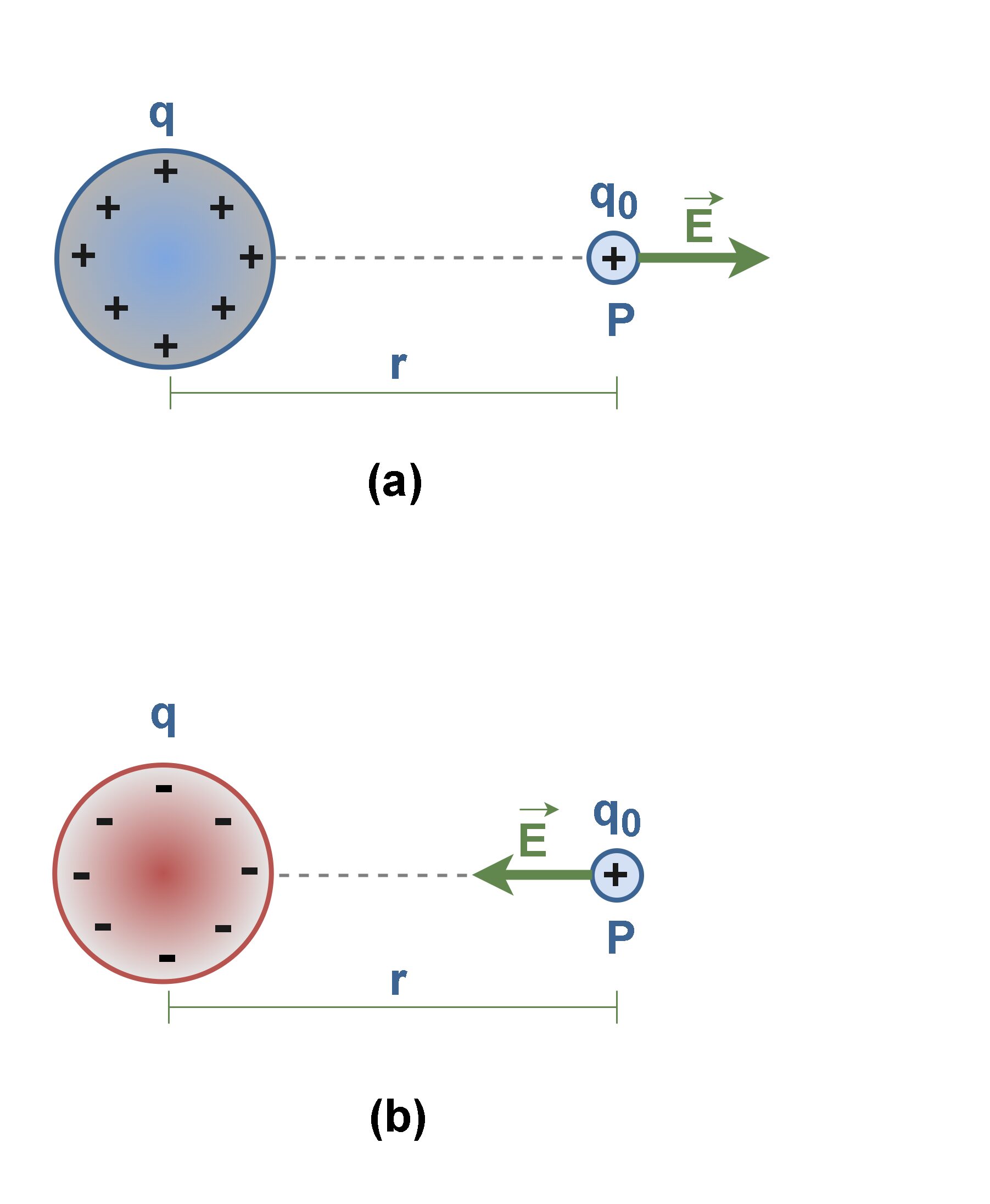
Figure 1 shows an object with a small positive charge q₀ placed at point P near a second object with a much larger positive charge q. In this case, the large charge q sets up an electric field at all points in the surrounding space, even if the space is a vacuum. This field has the property of causing a force to be exerted on another charge, called the test charge (q₀).

As shown in Figure 1, the direction of the electric field is the direction of the force that acts on a positive test charge q₀ placed in the field. From Figure 1 (a) it can be seen that if q is positive, the electric field at P points radially outward from q. Figure 1 (b) also shows that if q is negative, the electric field at P points radially inward to q.

 The electric field  which is produced by a charge q at the location of a small test charge q₀, is defined as the electric force  (exerted by q on q₀) divided by the value of the test charge q₀. Equation 1 explains this definition:

According to this definition, the units are those of force divided by charge. The unit in the SI system is Newton per Coulomb (N/C). We also measure this quantity by the practical unit of volts per meter (V/m).  The electric field always has the same direction as the electric force on the test charge.

Conceptually and experimentally, the test charge q₀ must be very small so it doesn’t cause any significant influence on the behavior of the main charge creating the electric field. It is possible to express the quantity in a different equation. We may apply Coulomb’s law for two charges of q and q₀ in Figure 1, the electric force will then be obtained by Equation 2:

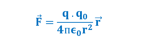
In Equation 2, r is the distance between the centers of two charges q and q₀, and the unit radius vector governs the direction of force from q to q₀.

Equation 3 can be concluded from Equations 1 and 2 to find another way to calculate the magnitude of the electric field created by the charge q:

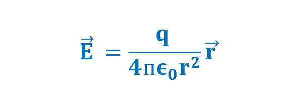
Here, the test charge q₀ has been omitted from the numerator and the denominator of the fraction. In these equations, it is assumed that the medium is air or vacuum.

Permittivity (ε) generally describes the effect of material in determining the electric field in response to electric charge. The permittivity of air is only slightly greater than that of free space and can usually be assumed to be equal. Thus, in free space (a perfect vacuum) we find that. In most other materials, the permittivity is significantly greater; that is, the same charge results in a weaker electric field intensity.

As Equation 3 indicates, an electric field at a given point in space depends only on the charge q setting up the field and the distance r from that object to the specific point (P). As a result, we can say that an electric field exists at point P in space whether there is a test charge at P or not.

Electric Field Lines

Michael Faraday, who introduced the idea of electric fields in the 19th century, envisioned lines in the space around any given charged object. These are called electric field lines.

Figure 2 gives an example in which a sphere is uniformly covered with a negative charge:

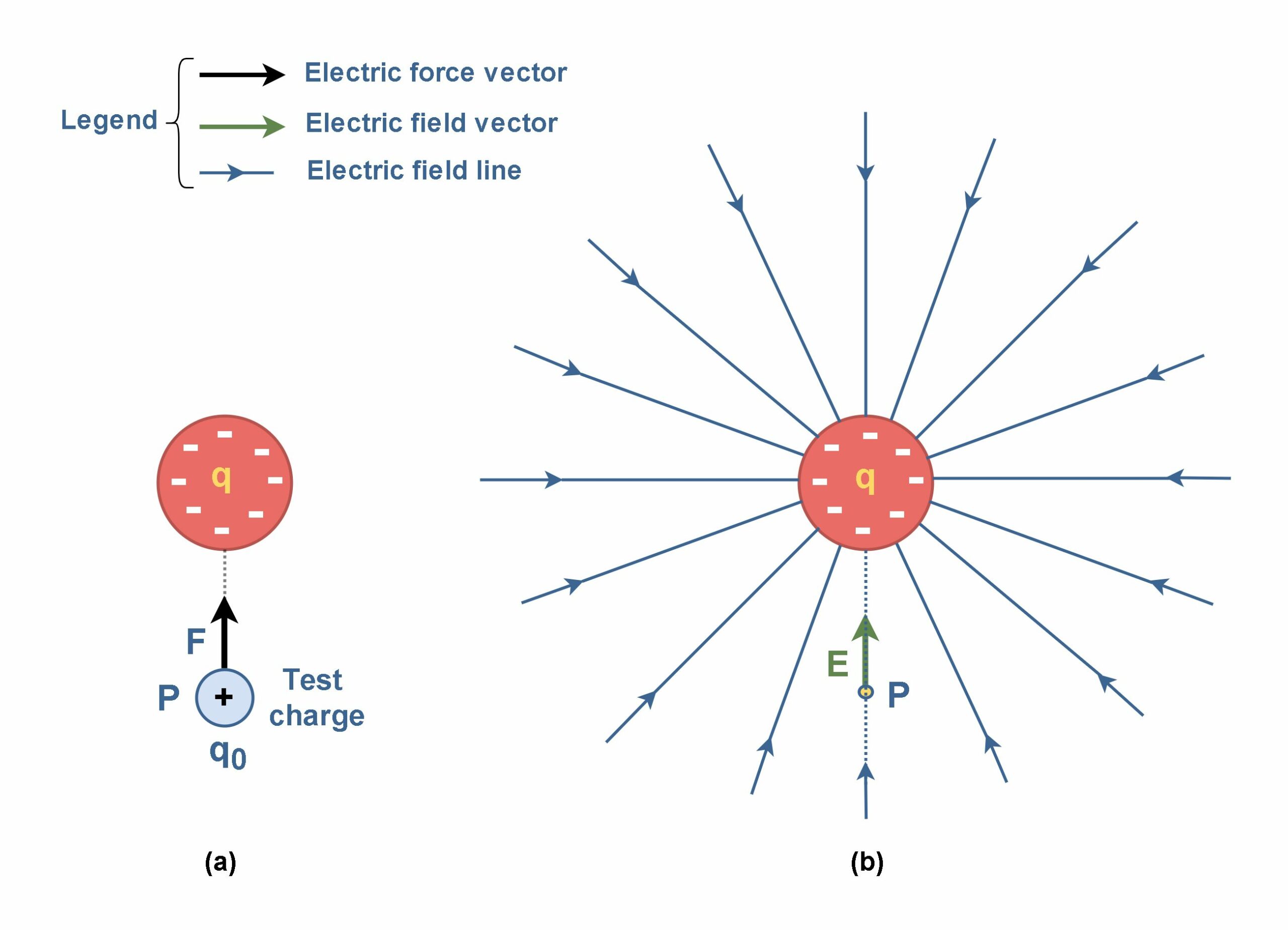
Figure 2(a) shows that if we place a positive test charge at any point around the sphere, an electrostatic force pulls on it toward the center of the sphere; because the negative charge attracts a positive test charge.  Thus, at every point around the sphere, an electric field vector points radially inward to the sphere’s center. Therefore, the electric field lines for a negative charge are also directed toward the charge.

One way to visualize the electric field is to draw field lines at different positions in space surrounding the charge q as shown in Figure 2(b). In fact, we could create a map in which every position in space surrounding the electric charge is assigned a vector that describes the force a test charge would experience if it were placed there. At any point, such as the one shown, the direction of the field line through the point matches the direction of the electric field vector.

This two-dimensional drawing contains only the field lines that lie in the plane containing the main charge (q) and the test charge (q₀). If the sphere in Figure 2 were uniformly covered with a positive charge, the electric field vectors at all points around it would be radially outward. Thus, the electric field lines would be directed radially outward from the charge in all directions of space.

The rules for drawing electric field lines for any charge distribution follow directly from the relationship between electric field lines and electric field vectors:

1. At any point, the electric field vector must be tangent to the electric field line through that point and in the same direction.
2. The lines must begin on positive charges and end on negative charges in space. However, some lines will begin or end infinitely far away, appearing to originate from or terminate on distant electric charges.
3. No two field lines can cross each other.
4. The number of lines per unit area drawn leaving a positive charge or ending on a negative charge is proportional to the magnitude of the field at that point. This means that a greater density of lines indicates a greater magnitude. Note that the electric field intensity E is large when the field lines are close together and small when the lines are far apart.

Figure 3 shows the field lines for two particles with equal positive charges:

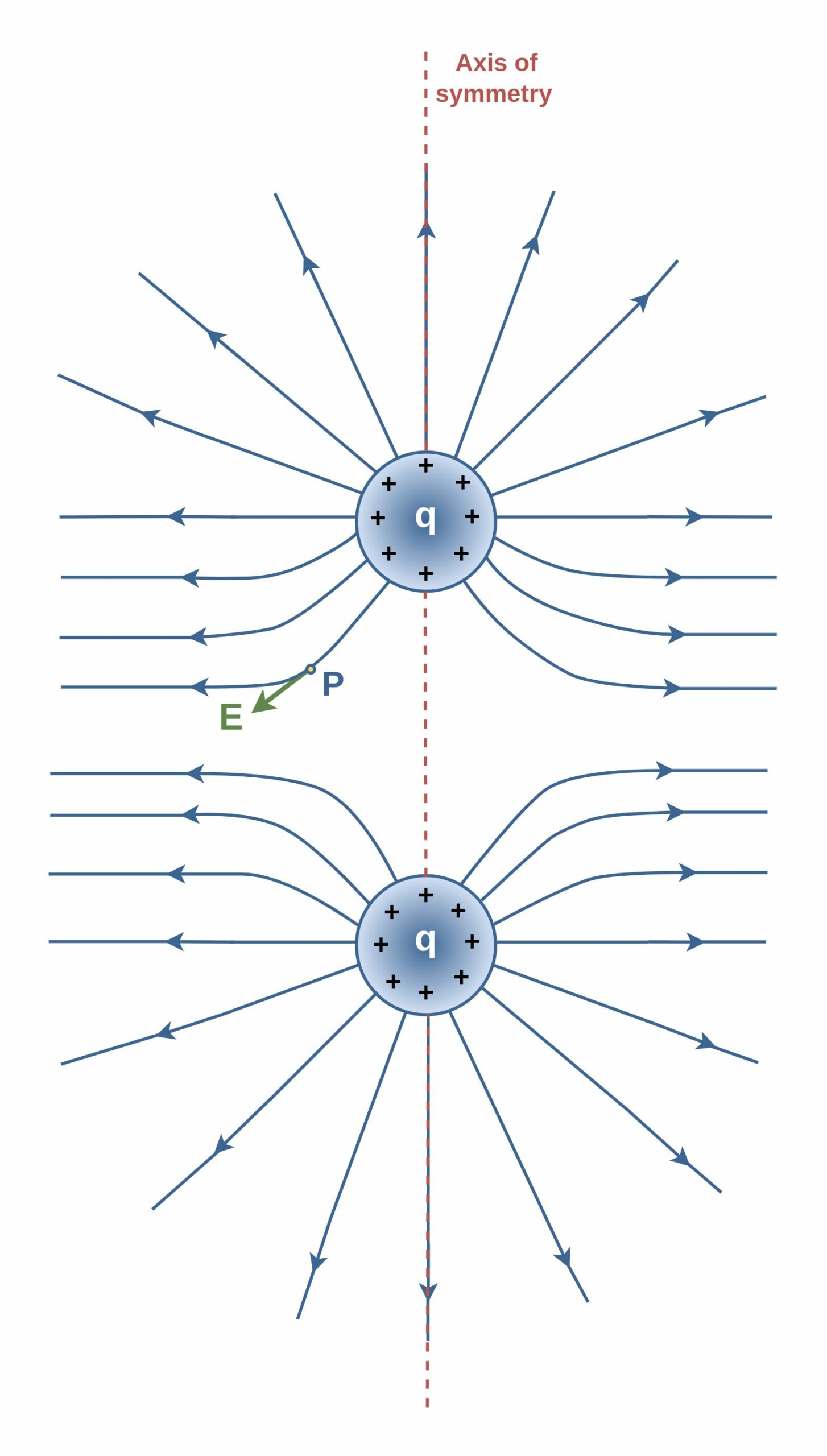
It can be seen that close to each charge, the lines are naturally nearly radial. However, the field lines are curved in other regions, especially in the space between charges. Nonetheless, the above-mentioned rules are still held.  The electric field vector at any given point must be tangent to the field line at that point and in the same direction, as shown for the vector at point P. Additionally, note that the lines are closer together as they approach the charges, indicating that the strength of the field is increasing. Equation 3 verifies that smaller r causes stronger E.

To imagine the full three-dimensional pattern of field lines around the particles, mentally rotate the pattern in Figure 3 around the axis of symmetry, which is a vertical line passing through both particles.

The same number of lines emerges from each charge because the charges are equal in magnitude. At great distances from the charges, the electric field is approximately equal to that of a single-point charge of magnitude 2q. The bell-shaped electric field lines between the charges reflect the repulsive nature of the electric force between like charges. Additionally, the low density of field lines between the charges indicates a weak field in this region.

The Electric Field Due To An Electric Dipole

Figure 4 shows the pattern of electric field lines for two particles that have the same charge magnitude (q), but opposite signs. This configuration is a very common and important arrangement known as an electric dipole.

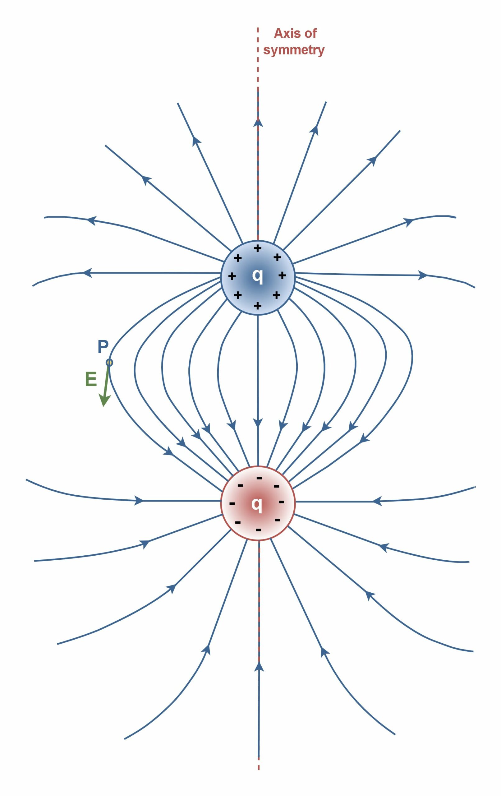
Figure 4 illustrates the symmetric electric field lines for an electric dipole. Note that the number of lines that begin at the positive charge must equal the number that terminates at the negative charge. At points very near either charge, the lines are nearly radial. The high density of lines between the charges indicates a strong electric field in this region, unlike the condition of two positive charges in Figure 3.

Figure 5 presents an example of an electric dipole with 2 charges +q and -q separated by distance d along the dipole axis, which serves as an axis of symmetry.  We focus our attention on the magnitude and direction of the electric field at an arbitrary point P along the dipole axis, at a distance z from the dipole’s midpoint. Figure 5 illustrates each particle’s electric fields set up at P (field lines are not plotted for simplicity).

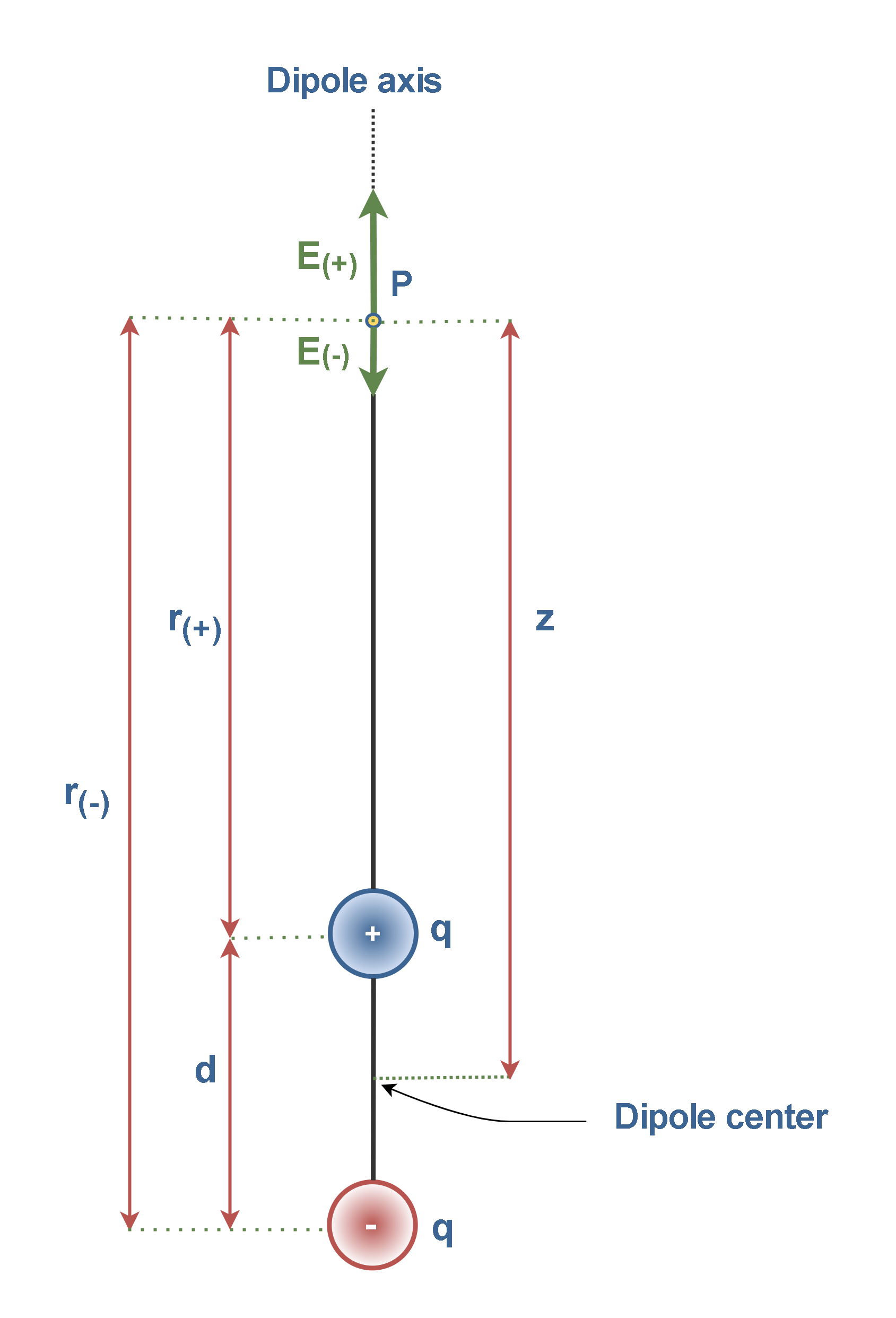
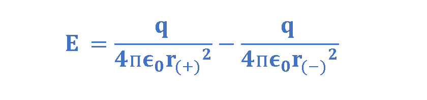
At the observation point P in the positive direction of the dipole axis, the closer particle with charge +q sets up field E₍₊₎ (directly away from the dipole center). The farther particle with charge -q sets up a smaller field E_(-) in the negative direction (directly toward the dipole center). We can find the net field at P by using Equation 3. However, because the field vectors are along the same axis, let’s indicate the vector directions with plus and minus signs. Then we can write the magnitude of the net field at P using the superposition principle as Equation 4:

We use Equation 3 to calculate the resultant electric field intensity, as shown by Equation 5:

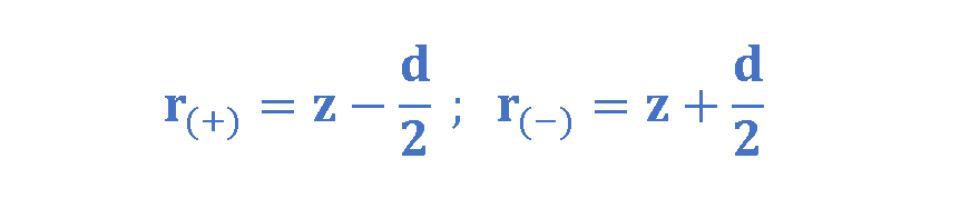
We also utilize the relationships between distances of r₍₊₎ (the distance between the positive charge and P) and r_(-) (the distance between the negative charge and P), d (the distance between charges) and z (the distance between the dipole center and the measurement point P) in Equation 6:

In most of applications, we are usually interested in the electrical effect of a dipole only at distances that are large compared with the dimensions of the dipole — that is, at distances such that z >> d. At such large distances, we have d/z << 1. Thus, we can calculate E by this approximation and conclude Equation 7:

Therefore, the electric field strength (E) due to a dipole at a far distance, is always proportional to the dipole moment (q × d) and inversely proportional to the cube of the distance (z³). The dipole moment is the product of the charge and distance between the two charges, and it is essentially a vector quantity.

Inspection of Equation 7 shows that if you double the distance of a point from a dipole, the electric field at the point drops by a factor of 8 (= 2³). However, if you double the distance from a single point charge, (see Equation 3), the electric field drops only by a factor of 4 (= 2²). Thus, the electric field of a dipole decreases more rapidly with distance than does the electric field of a single charge.

The physical reason for this rapid decrease in electric field for a dipole is that from distant points a dipole looks like two particles that almost coincide. Thus, because they have charges of equal magnitude but opposite signs, their electric fields at distant points almost — but not quite — cancel each other, resulting in a minimal resultant field effect of the charge combination.

Summary

• An electric field exists at a point if a test charge at that point is subject to an electric force there.
• We can represent the electric field with electric field lines. The electric field lines are essentially a map of electric field vectors. The direction of each line then represents the direction of the electric field at that point.
• The direction of electric field lines is from positive charges toward negative charges. Electric field lines originate in positive charges and then extend away toward negative charges and terminate there.
• Essentially, permittivity is a constant that depends on the material.
• At every point around a positively charged sphere, an electric field vector points radially outward from the center of the sphere. Because a positive test charge placed in this field would be repelled by the charge q, the lines are directed radially away from the positive charge.
• In either case, the lines are radial and extend all the way to infinity.
• Closer spacing of field lines means a larger field magnitude.
• The charge configuration of two-point charges of equal magnitude but the opposite sign is called an electric dipole.

Please follow and like us: