An Overview On Electrostatics – Electric Potential In Nonuniform Fields

Electric Potential Due To Point Charges

In physics, electric fields are regions in space where an electric force is experienced by a charged object due to the presence of another charged object. These fields can be either uniform or non-uniform. A uniform field is one where the field strength (or the force) is the same at every point in the field. This means that the magnitude and direction of the field are constant throughout. We will consider these types of fields in the next article.

Non-uniform fields are those where the field strength and direction vary from point to point. This means that the magnitude and direction of the field can change depending on different positions in the field. The electric field due to a point charge is an example of a non-uniform field since it decreases with distance away from the source charge. Recall that a point charge is an electric charge considered to exist at a single point, and thus having neither area nor volume, i.e., an idealized mathematical concept.

Consider the case of a nonuniform electric field such as exists in the vicinity of the positive point charge Q in Figure 1. Let us assume a positive test charge q₀ is located at point P in the field E associated with the charge Q.

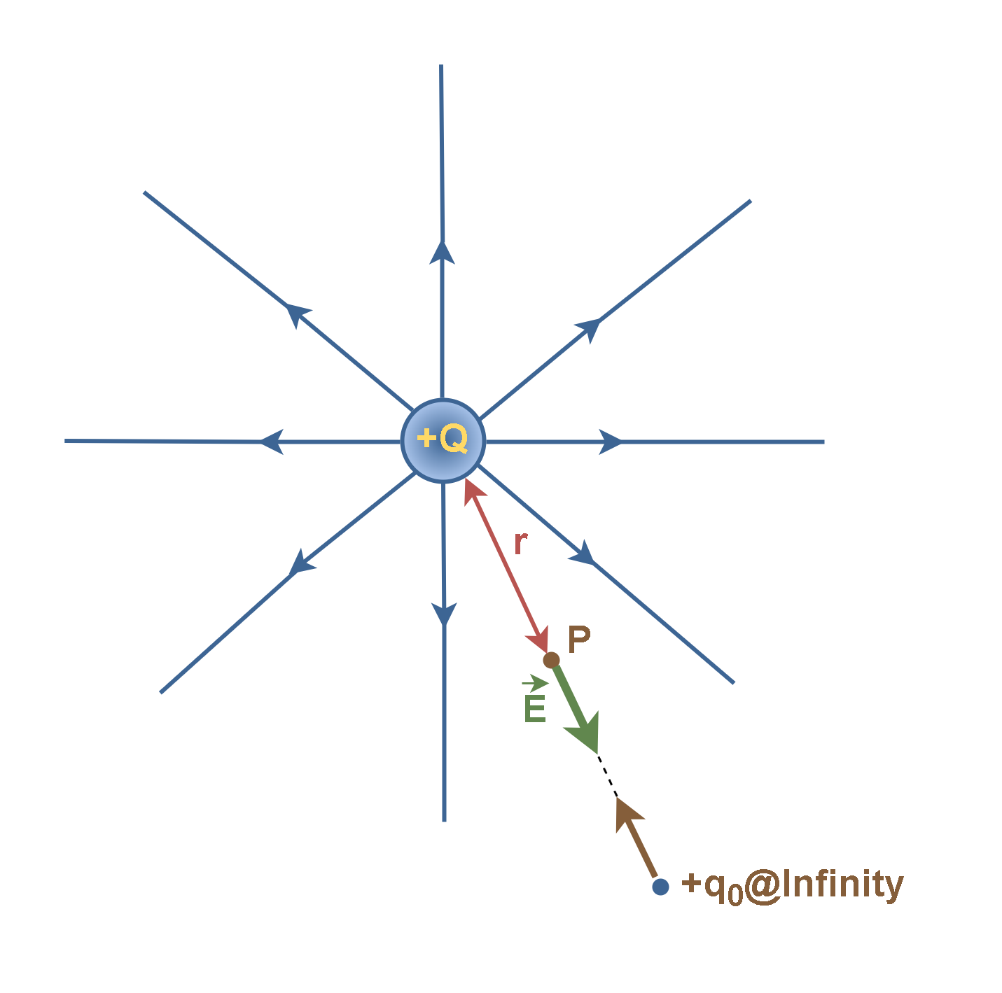
Naturally, there is a nonuniform electric field at point P caused by the charge Q, and so there is an electric force F at point P which is exerted to the test charge q₀ as it explained by Equation 1:

Generally, Field lines indicate the directions of the force on a positive test charge introduced into the field. If the test charge is released in a field, it moves in the direction of field lines in each position. In the case of a point charge Q, it moves radially away from Q, so that the field lines are radial, like the spokes of a wheel. The field intensity also varies inversely as the square of the distance from Q. For this reason, In Figure 1 the field lines become more widely separated as the distance ‘r’ increases.

In Figure 1 configuration, we want to find the potential energy U associated with the test charge at point P. First, we need a reference configuration for zero potential energy (U = 0). A reasonable choice is for the test charge q₀ to be infinitely far from the charge Q, because then there is no interaction between charges.

We know that if we want to move the test charge q₀ against the electric force F, it requires physical work. The work done by the applied force F on the charge q₀ changes its potential energy U. Then, we assume that we bring the test charge from infinity to point P in the configuration of Figure 1.

The electric potential V at the point P in space is defined as the work done in bringing a positive test charge q₀ from infinity to that point, divided by the magnitude of the charge. Let’s use the notation ∞ for W to emphasize that the test charge is brought in from infinity and also use a negative sign for W_∞ because it is done opposite to the electric force F. Then, the electric potential V at point P is given by Equation 2:

So, the electric potential V is the amount of potential energy per unit charge. The charge Q sets up this potential V at point P regardless of whether the test charge happens to be there. The work and thus the potential energy can be positive or negative depending on the sign of the charge Q.

From Equation 2 we see that V is a scalar quantity (because there is no direction associated with potential energy or charge) and can be positive or negative (because potential energy and charge have signs). The work W_∞ done by the field is also scalar and path-independent.

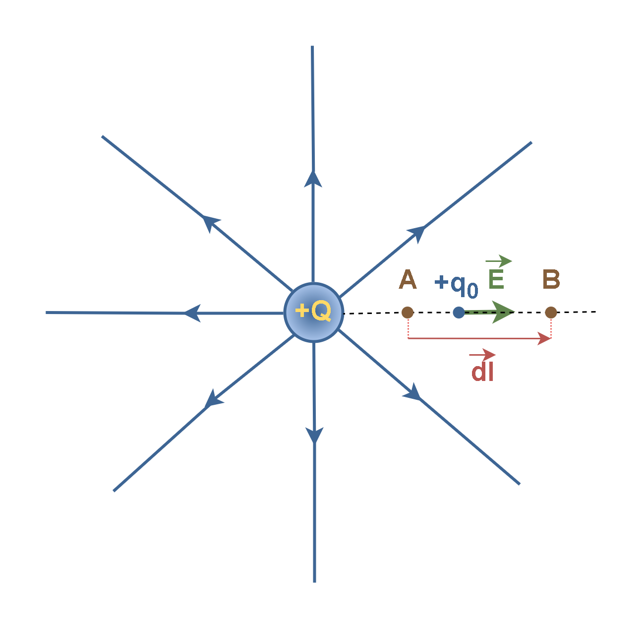
If the test charge q₀ moves from an initial point A to a second point B in the electric field of a charged object, as depicted in Figure 2, the electric potential changes by ΔV = V_B – V_A. We can relate the potential energy change ΔU to the work W_AB done by the electric force as the particle moves from A to B by substituting from Equation 2 to conclude Equation 3:

Generally, if the test charge q₀ moves between points A and B in the field, the work W_AB done is given by Equation 4:

where F is the electric force on the test charge and is the path vector which indicates the moving of the test charge q₀ between points A and B.

Because in our assumption the test charge q₀ moves between points A and B in the field E along a radial path, therefore, the vectors have the same direction, and the dot-product of vectors inside the integral in Equation 4 simply changes to the scalar product of magnitudes of the two vectors.

In our previous articles we have already calculated the intensity of electric field E based on Coulomb’s law as explained in Equation 5:

With this choice, simple mathematics can be used to show that by substituting Equation 5 in Equation 4 and Equation 2 and assuming that the point B is in infinity (V_B = 0), we can calculate the electric potential V_A. Finally, this electric potential created by a particle of charge Q at any radial distance r from the particle is given by Equation 6:

Generally, every charged object sets up an electric potential V_P at all points throughout its electric field. The electric field of a point charge extends throughout space, so its electric potential does, also. The zero point of electric potential could be taken anywhere but is usually taken to be an infinite distance from the charge, far from its influence and the influence of any other charges.

The SI unit of electric potential, which is also referred to as voltage drop, is ‘Joules per Coulomb’ or volt (V) after Alessandro Volta (1745-1827), an Italian physicist and chemist who was a pioneer of electricity, where 1 V = 1 J/C. it means 1 J of work must be done to move a 1-C charge between two points that are at a potential difference of 1 V.

Equation 6 shows that the electric potential (V_A) increases as the positive test charge q₀ moves closer to the point charge Q. This can be shown numerically if we assume (Q = +1.11 × 10^-9C = +1.11 nC). Now we can calculate the electric potential and the electric field in terms of different values of r. The results are provided in Table 1:

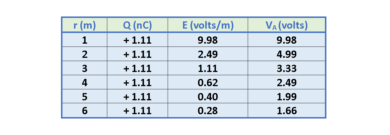
Figure 3 shows the plot of the electric field and the electric potential based on the numerical data in Table 1.

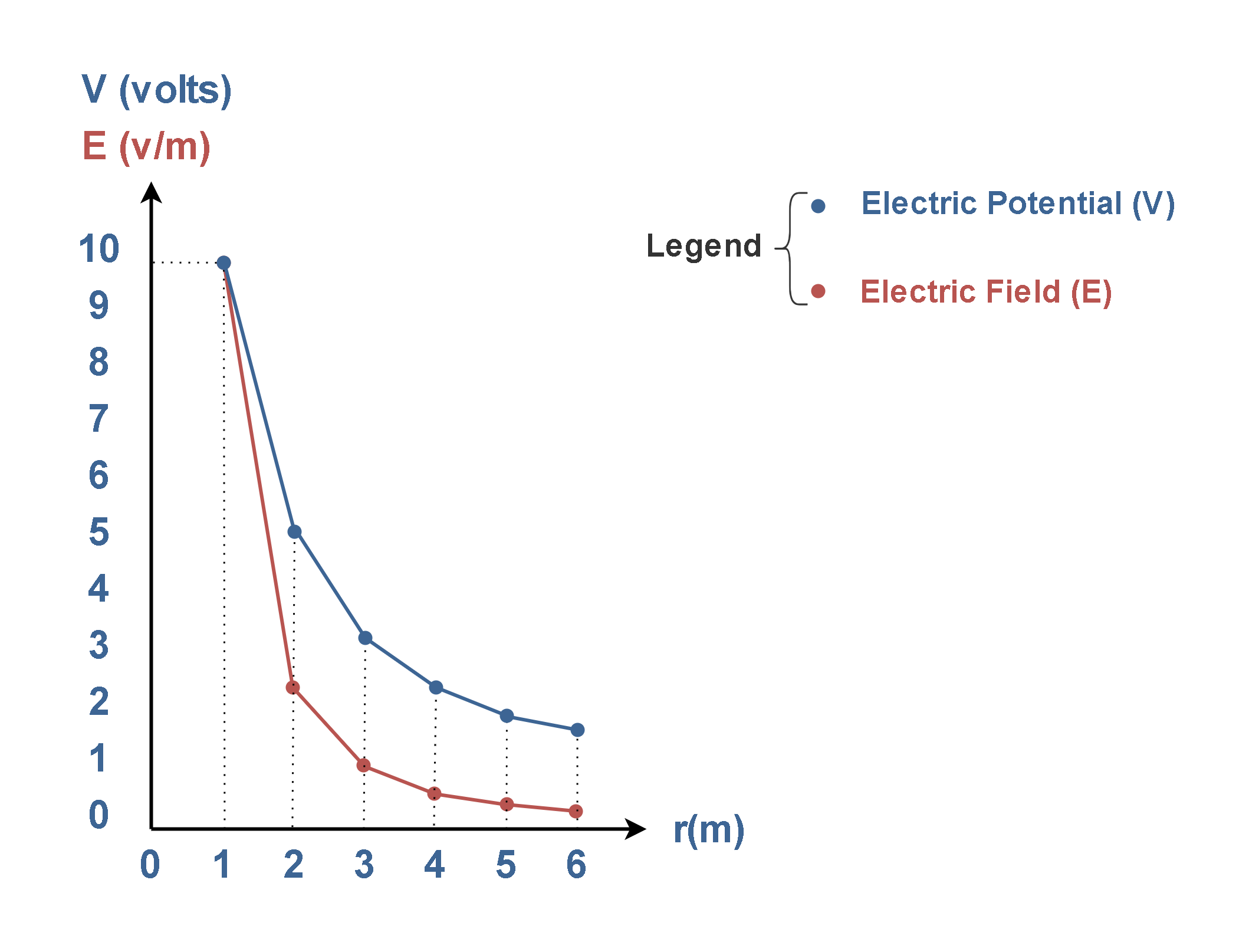
This visual representation summarizes the fundamental principles regarding how the electric potential and field strength vary with distance from a point charge source. Figure 3 confirms these key points:

1. The electric potential V (blue curve) decreases inversely with increasing r, following a 1/r dependence as described by Equation 6.
2. The electric field strength E (red curve) decreases more rapidly, following an inverse square 1/r² dependence as described by Equation 5.
3. At smaller values of r, both V and E have higher magnitudes since the test point is closer to the point charge source.
4. As r increases towards larger values, V decreases gradually while E drops off more sharply.

Electric Potential Due To A Group Of Charged Particles

We can find the net electric potential at a point due to a group of charged particles with the help of the superposition principle. It means the total electric potential at some point P due to several point charges is the algebraic sum of the electric potentials due to the individual charges. Compared to the electric field, it is simpler to sum several scalar quantities than to sum several vector quantities whose directions and components must be considered.

Figure 4 shows a configuration of 4 charged particles, q₁ to q₄, which are placed in corners of a square. We can calculate the electric potential at point P in the center of the square.

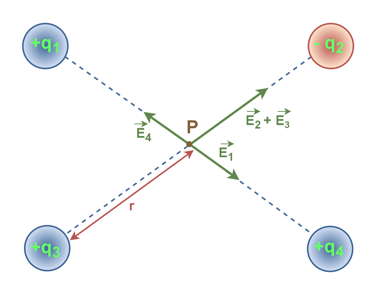
The electric field vectors (E1, E2, E3, E4) due to each charge are shown at the center point P. The distance ‘r’ from each charge to the center point P is also indicated in the diagram.

Recall that the electric potential created by a point charge Q is generally given by Equation 7 which is another form of Equation 6:

where, k_e = 8.9875 × 10⁹ (Nm²/C²) is the Coulomb’s constant.

Unlike electric field superposition, which involves a sum of vectors, the superposition of electric potentials simply requires evaluating a sum of scalars. Equation 8 gives the simple key to find the net electric potential in a general configuration of ‘n’ charged particles.

Here q_i is the value of the ith charge and r_i is the radial distance of the given point from the ith charge. In this configuration all the charges have equal distances to the point P. Using Equation 7, an algebraic sum with the plus or minus sign of the charge included, we calculate separately the potential resulting from each charge at the given point. Then we sum the potentials.

In our example with n = 4 charges in Figure 4, we assume the value of charges are: q₁ = +12nC, q_{2 =} -24nC, q₃ = +31nC, q₄ = +17nC and the distance between charges and point P is r = 0.919 m.

Thus, the net potential at point P is calculated by Equation 9:

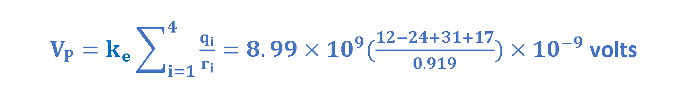
Finally, the net potential at point P is V = 352 volts! It may seem strange that a combination of such small changes can make such big voltage!

Equipotential Surfaces

An equipotential surface is the collection of points in space that are all at the same electric potential. The potential difference between any two points on an equipotential surface is zero. Hence, no work is required to move a charge on an equipotential surface. The electric field at every point of an equipotential surface is perpendicular to the surface.

Equipotential surfaces can be represented on a diagram by drawing two-dimensional equipotential contours. Figure 5 depicts the concentric circular equipotential contours (brown dotted circles) surrounding the positive point charge +Q.

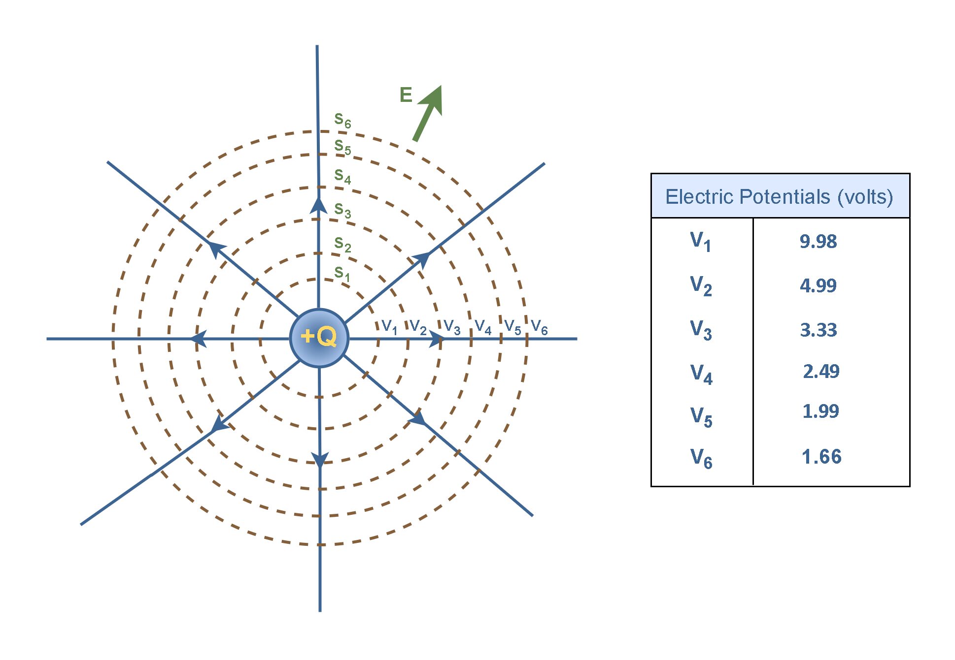
Following our previous example, if Q = +1.11 nC, the equipotential contours are plotted as S₁ to S₆. Each circle can be assigned a constant electric potential (V₁ to V₆) and the voltage values are provided in a table in Figure 5. These values are mapped to the different equipotential contours in the plot.

It is also to be noted that electric potentials rise in the opposite direction to E. As we start from the location of the charged object +Q and move outward, by increasing distance, the equipotential values decrease from 9.98 volts (V₁) to 1.66 volts (V₆) at the outermost circle.

This relation shows that, for a single-point charge, the potential is constant on any surface on which ‘r‘ is constant. Imagine that by rotating the two-dimensional plot in Figure 5 about the vertical axis, the complete three-dimensional plot is generated and the dashed circular equipotential lines in the present plot are changed to spherical equipotential surfaces. It follows that the equipotential surfaces of a point charge are a family of spheres centered on the point charge.

Summary

• If an electric field has the same magnitude and direction everywhere in a particular space, it is said to be uniform.
• A non-uniform electric field varies in magnitude according to different positions.
• The electric potential is the amount of potential energy per unit charge when a positive test charge is brought in from infinity.
• The word ‘Potential’ at a point is a scalar quantity.
• The amount of work per unit charge is equal to the force per unit charge (or field intensity E) times the distance through which the charge is moved.
• Voltage is another term for electric potential, it measures the difference in electric potential between two points.
• The electric potential difference between points A and B, (V_B-V_A) is defined to be the change in potential energy of a charge q moved from A to B, divided by the charge.
• The SI unit of electric potential is the joule per coulomb (J/C), called the volt (V).
• Because the electric force is conservative, the change in potential energy ΔU between two points is the same for all paths between those points (it is path-independent).
• The electric potential of two or more charges is obtained by applying the superposition principle.
• A surface on which all points are at the same potential is called an equipotential surface.
• Equipotential surfaces are always perpendicular to electric field lines.
• It is obvious that with increasing r, the electric potential V_A associated with the point charge Q decreases as 1/r, in contrast to the magnitude of the charge’s electric field, which decreases as 1/r².

Please follow and like us: