Electric Displacement and Electrostatic Energy

Electric Displacement

Around 1837, Michael Faraday, the director of the Royal Society in London, became interested in static electric fields and the effect of various insulating (or dielectric) materials on these fields. He constructed a pair of concentric metallic spheres, the outer one consisting of two hemispheres that could be firmly clamped together. He also prepared shells of dielectric material that would occupy the entire volume between the concentric spheres (like the structure depicted in Figure 1).

Faraday found that the total charge on the outer metallic sphere was equal in magnitude to the original charge placed on the inner sphere, and this was true regardless of the type of dielectric material separating the two spheres. He concluded that there was some sort of electric displacement from the inner sphere to the outer, which was independent of the medium.

Nowadays, we know that a field applied to an insulator may produce no migration of charge. However, it can produce a polarization of the insulator (or dielectric), i.e., a displacement of the charges concerning their equilibrium positions.

For a better understanding of Faraday’s experiments, let’s consider Figure 1 with an inner metal sphere of radius ‘a’ and an outer metal sphere of radius ‘b’, with charges of +Q and -Q, respectively.

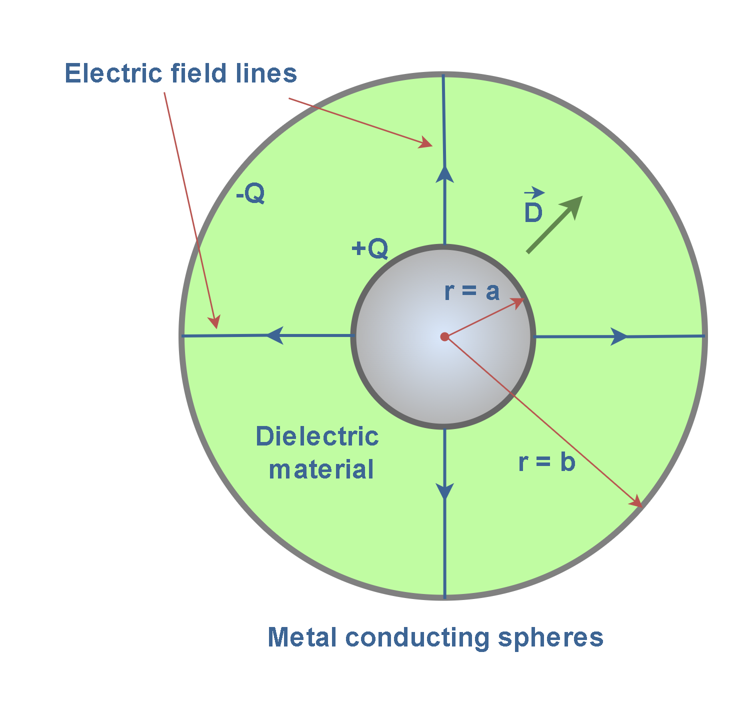
According to Faraday’s findings, we know there is a direct proportionality between the electric flux φ_E and the charge on the inner sphere in this structure. At the surface of the inner sphere, electric flux lines φ_E are produced by the charge Q distributed uniformly over a surface having an area of (4πa²) square meter. The paths of electric flux extending from the inner sphere to the outer sphere are indicated in Figure 1. The field lines are symmetrically distributed streamlines drawn radially from the inner sphere to the outer one (just some of them are plotted for simplicity).

The density of the flux at the inner surface is (φ_E /4πa²), and this is an important new quantity. The number of electric field lines flowing perpendicularly through a unit surface area is called electric flux density and it is denoted by D. The electric flux density D is a vector field and its direction at a point is the direction of the flux lines at that point (as shown in Figure 1), and its magnitude is given by the number of flux lines crossing a surface normal to the lines divided by the surface area. It is measured in coulombs per square meter (C/m²).

Electric flux density has the alternate names of electric induction or electric displacement that is more descriptive. Essentially, electric displacement (D) is a concept in electromagnetism that describes how electric fields interact with materials. In simple terms, the electric displacement (flux density) D represents the amount of electric field passing through a unit area of a material.

The constitutional relation between electric displacement D and electric field E in vacuum or free space is explained in Equation 1.

where, ϵ₀​ is the electric permittivity of vacuum (or free space), with the value of 8.85 × 10⁻¹² F/m. Since ϵ₀ is a very small positive number (less than 1), in free space, the corresponding D field will always have a smaller magnitude than E.

In materials other than a vacuum, the permittivity ϵ can be more complex and include the effects of the material’s polarization. If we put a piece of dielectric into an external field E, the field will polarize the material. This polarization will produce its internal field, which then contributes to the total field.

If the properties of the material do not depend upon position, the material is said to be homogeneous. If the response of the material is the same for all directions of the electric field vector, it is called isotropic. A material is called linear if the ratio of the response of the material’s polarization to the field E is independent of the amplitude of the polarizing field.

In our discussion, the media is assumed to be homogeneous, isotropic and linear. For such dielectric materials, the permittivity ϵ can be expressed as Equation 2:

where the constant χ_e is called the electric susceptibility of the material and it is dimensionless. The electric susceptibility indicates the degree of polarization of a dielectric material in response to an applied electric field. The value of χ_e depends on the microscopic structure of the substance and also on external conditions such as temperature. In a vacuum, where there is no matter to polarize, the susceptibility is zero, and the permittivity ϵ is equal to ϵ₀​.

The general relationship between electric displacement D, the external electric field E, and electric permittivity ϵ in dielectric materials is given by Equation 3:

We know that the polarization of a dielectric ordinarily results from an electric field, which lines up the atomic or molecular dipoles. For many substances, the polarization is proportional to the field, provided E is not too strong. The electric polarization (or polarization density) vector, which is denoted by, represents the volumetric density of permanent or induced electric dipole moments in a dielectric material. Equation 4 defines P:

Essentially, the vector P describes the overall alignment of electric dipoles in a material in response to an applied electric field E. It is a vector quantity that is measured in Coulombs per square meter (C/m²) in SI units.

Therefore, in comparison to Equation 1, when a material medium is present, one has to add the contribution to D by the polarization vector. Then, D is concluded with a new general definition as Equation 5 explains:

We cannot compute directly from Equation 5. The simplest approach is to begin with the displacement D.

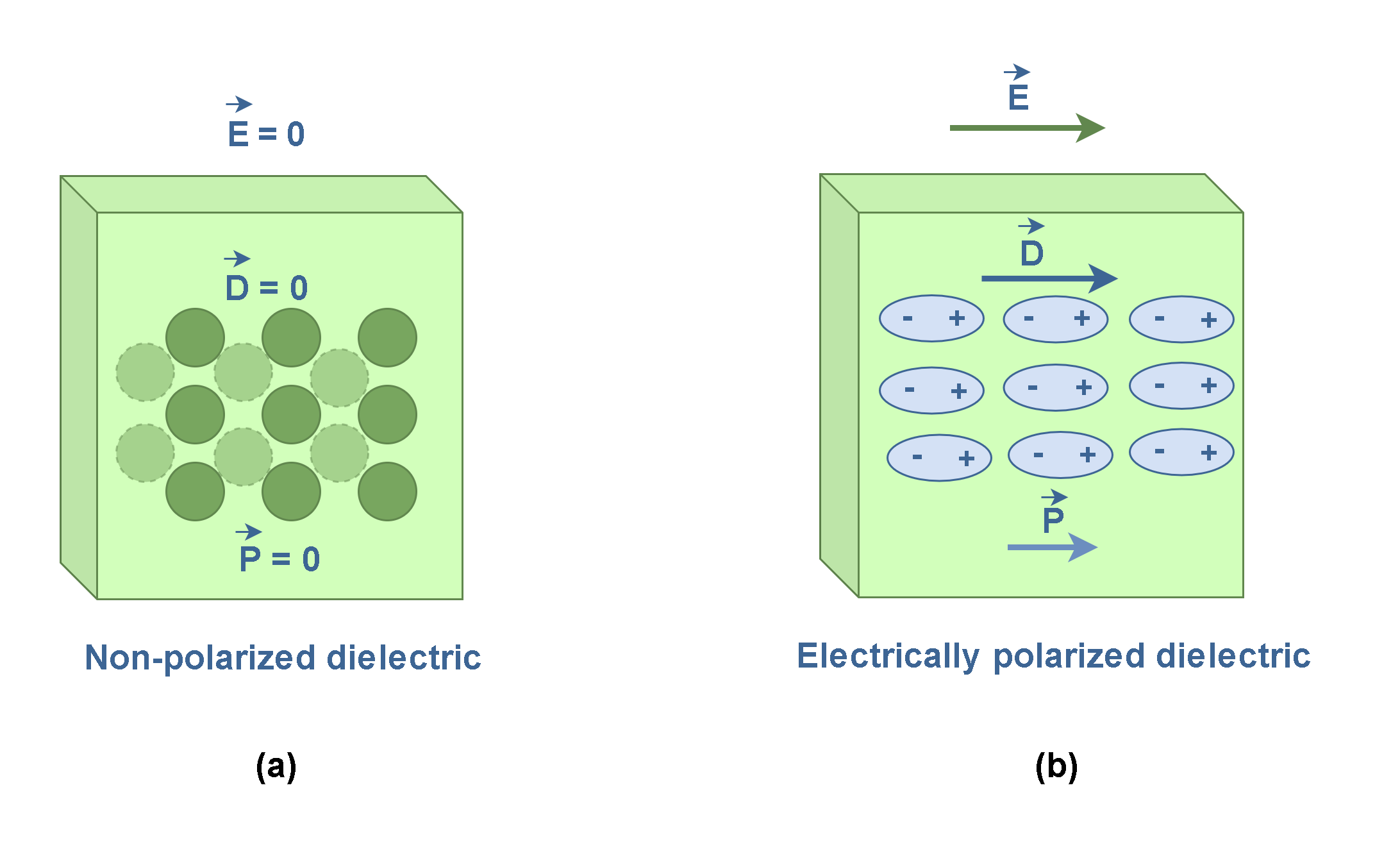
Figure 2 depicts the molecular orientation of a piece of dielectric in 2 conditions: (a) there is not any applied external electric field E, thus, the molecules are neutral and the field vectors of D are zero inside the dielectric. (b) there is an applied electric field E  and the polarized molecules of the dielectric are oriented in the direction of the external field while the field vectors of D and P are not zero and have finite values.

Finally, by comparison of Equation 2 and Equation 3, we can define the electric displacement as in Equation 6:

where ϵ_r is the relative permittivity and κ is similarly called the dielectric constant. We have already considered them as equal parameters.

Thus, the factor of proportionality relating electric displacement D and electric field E in a dielectric is simply the dielectric constant κ of the medium times the electric permittivity of vacuum ϵ₀.

Gauss’s Law In The Presence Of Dielectrics

We have already discussed that Gauss’s Law, named after the German mathematician Carl Friedrich Gauss, is a fundamental concept in electromagnetism that describes the relationship between electric charges and the electric field they produce. The law states that the total electric flux through a closed surface is proportional to the enclosed charge.

In vacuum or free space, Gauss’s Law states that the electric flux through a closed surface (called Gaussian surface) is proportional to the enclosed charge as explained in Equation 7:

where φ_E is the electric flux, E is the electric field, dA is an infinitesimal area element, and Q_inside is the enclosed charge in the closed surface.

When a dielectric material is placed in an electric field E, the positive and negative charges within the material are displaced, creating bound charges on surfaces.

Equation 8 calculates the total charge inside the Gaussian surface after polarization:

The free charges (Q_free) are the excess charges that can move freely. They might consist of electrons on a conductor or ions embedded in the dielectric material or whatever; these charges are not a result of polarization. While bound charges (Q_bound) are that arise from the polarization of the dielectric material.

In the presence of dielectrics, Gauss’s Law must be modified to account for the bound charges. This is done by introducing the concept of electric displacement field (D) which is related to the external electric field (E) and the polarization (P) of the dielectric material.

The modified Gauss’s Law in the presence of dielectrics is explained in terms of the vector D in Equation 9:

where D is the electric displacement (or flux density), and Q_free is the free charge enclosed by the Gaussian surface. Although in this form of Gauss’s Law, just the free charges are taken into account, bound charges are already accounted for in the electric displacement field D.

In particular, whenever the requisite symmetry is present, we can immediately calculate D by the standard Gauss’s law methods. After finding D it would be easy to calculate the electric field E in each place.

Example Of Gauss’s Law In The Presence Of Dielectrics In A Capacitor

Figure 3 shows a parallel-plate capacitor of plate area A, both with air (a) and with a dielectric of relative permittivity κ (b). We assume that the charge amount of Q on the plates is the same in both situations.

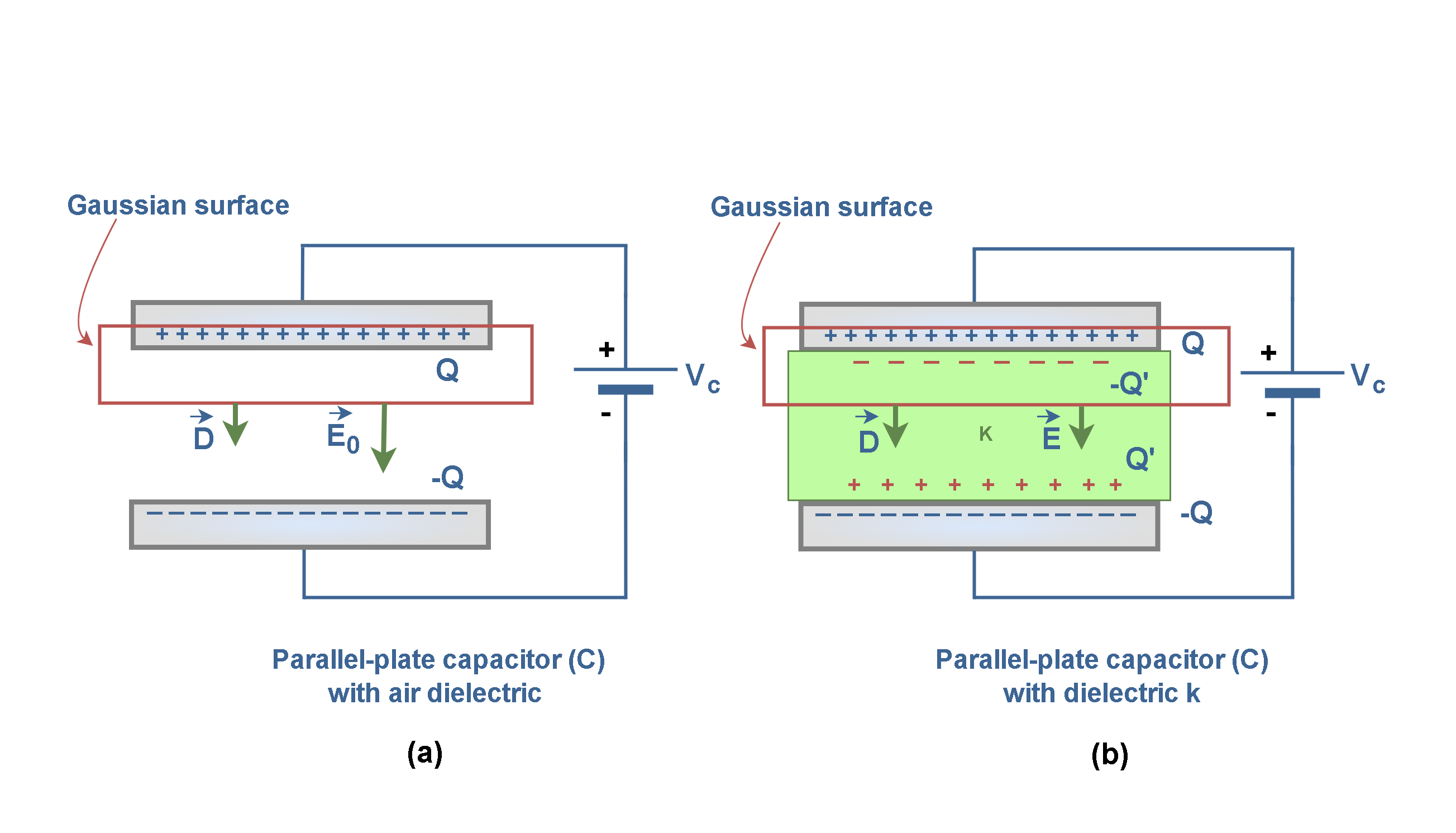
For the situation of Figure 3a, without a dielectric, we can find the electric field E₀ between the plates. We enclose the positive charge Q on the top plate with a Gaussian surface and then apply Gauss’s law. Letting D represent the magnitude of the electric displacement, we can use Equation 10 to find it:

By knowing the values of q and A, the value of D can be simply calculated. From this, we can then derive Equation 11 to find E₀ as the magnitude of the field E₀:

Note that in Figure 3b, the field between the metal plates induces charges on the faces of the dielectric slab. We can find the electric field between the plates (and within the dielectric slab) by using the same Gaussian surface. Note that in Figure 3b, with the dielectric in place, the field between the plates induces charges on the faces of the dielectric.

In Figure 3b, the surface encloses two types of charge: the free charge +Q on the top plate, and the induced charge -Q’ on the top face of the dielectric. Thus, the net charge enclosed by the upper Gaussian surface is (Q – Q’). The magnitude Q’ of the induced surface charge is less than that of the free charge q and is zero if no dielectric is present.

So, based on Equation 9, Gauss’s law now gives again the result of Equation 10 for finding D the same. The charge enclosed by the Gaussian surface is now taken to be the free charge Q only. The induced surface charge Q’ is ignored on the right side of Equation 10, having already been taken into account by introducing the dielectric constant κ. For this reason, D remains the same while E changes.

Thus, the result for calculating E is different and explained by Equation 12:

The bound charges in the dielectric create an induced electric field, which opposes the external electric field E₀. Therefore, the net electric field inside a dielectric E is reduced compared to free space by a factor of κ.

Advantages Of Using The Electric Displacement (D) In Gauss’s Law

• In essence, the modified Gauss’s Law with D simplifies our calculations by incorporating the complex behavior of the dielectric material into a single field quantity, allowing us to relate it directly to the free charges in the system. Free charges are the entities that we can control.
• D is continuous across dielectric boundaries, making it easier to solve problems involving interfaces between different materials (boundary conditions).
• D provides a macroscopic description of the electric field in materials, averaging out microscopic variations (like polarization P) due to individual small dipoles in dielectrics.
• This formulation of Gauss’s Law allows us to analyze electric fields in and around dielectric materials, which is crucial for many practical applications in electrical engineering; such as capacitor design and analyzing electrostatic shielding.

Therefore, by using the displacement vector in Gauss’s Law, we gain a powerful tool for analyzing electric fields in and around linear dielectric materials, simplifying many complex electrostatic problems and providing deeper insights into material behavior in electric fields.

Electrostatic Energy

Generally, electrostatic energy is the potential energy caused by electric fields of non-moving electric charges. The stored energy can be described in terms of the elastic quality of the electric field, similar to the viewpoint that a spring stores the energy in a mechanical system.

The energy associated with a charge distribution can be expressed in terms of the fields alone. Generally, the total energy in the fields can be calculated by integrating the fields over the volume that encloses the charge distribution as explained in Equation 13:

where W_e is the electrostatic energy of a charge distribution. W_e is measured in units of Joules.

Consider a structure consisting of two perfect conductors, both fixed in position and separated by an ideal dielectric. This could be a capacitor that can store energy. It could also be one of a variety of capacitive structures that are not explicitly intended to be a capacitor – for example, a printed circuit board.

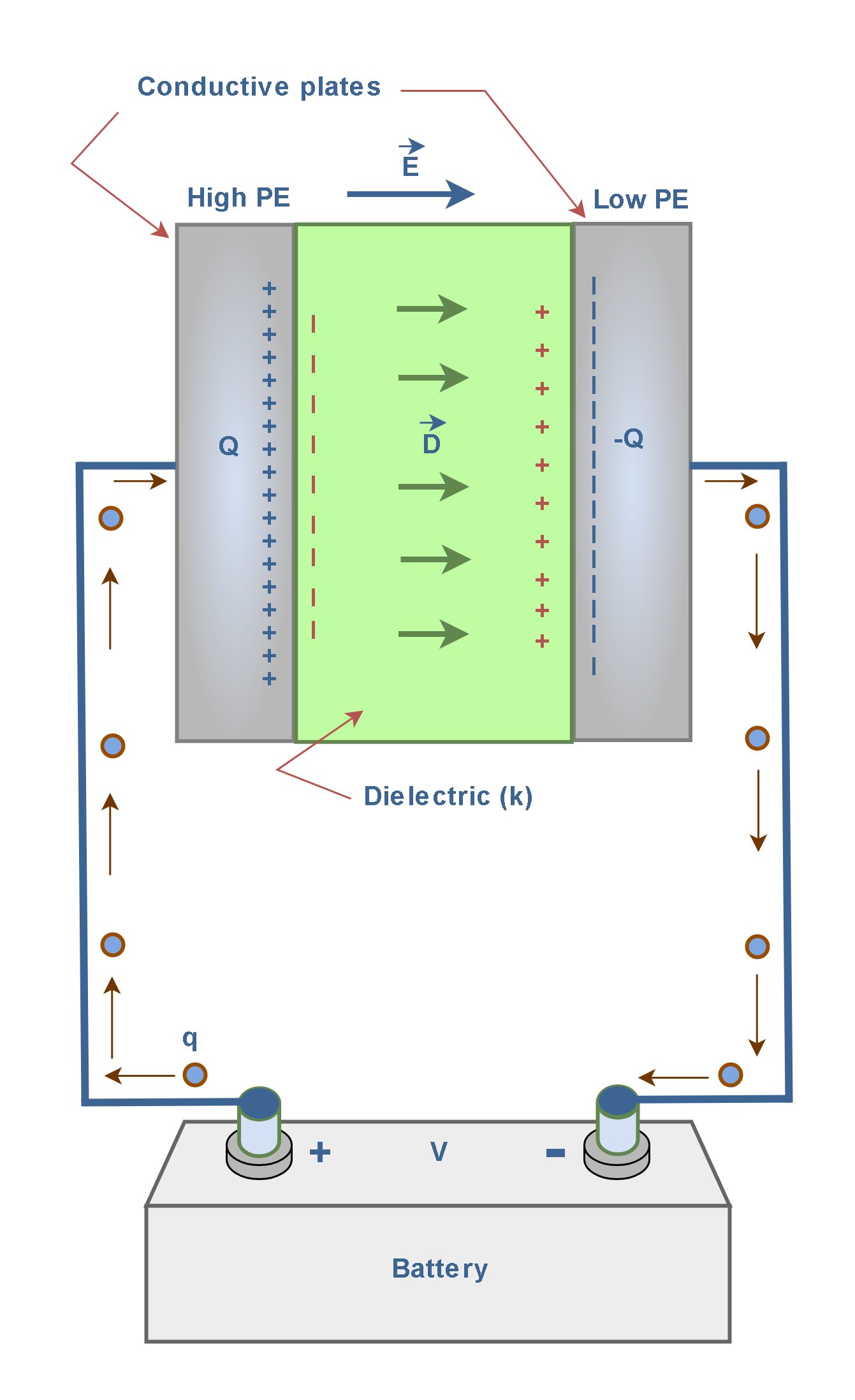
In a simple parallel-plate capacitor (C), when a potential difference V is applied between the two conducting planes, a positive free charge +Q will appear on the surface of the conductor at the higher potential (HP), and a negative free charge -Q will appear on the surface of the conductor at the lower potential (LP). Figure 4 shows such a structure.

The energy stored in the electric field in such capacitors can then be simply calculated by Equation 14. Here, W_e is the electrostatic energy in terms of the potential difference V between the capacitor plates.

where Q is the total free charge accumulated on each plate and C is the capacitance of this structure. When the charge is expressed in coulombs, the potential difference is expressed in volts, and the capacitance is expressed in farads, this relation gives the energy in joules.

Essentially, finding the potential energy stored in the electric field associated with the charges is important in modern electronic systems. For example, any system that includes capacitance uses some fraction of the energy delivered by the power supply (like the battery in Figure 4) to charge the capacitive structures. For this reason, there is a limit to the maximum energy (or charge) that can be stored in a capacitor.

Summary

• When free charges are placed near or in contact with a dielectric, the external electric field polarizes the atoms or molecules of the dielectric.
• This polarization produces bound charges within the material.
• The term “free charge” refers to charges that can move in response to changes in the electric potential.
• The resultant electric field is the sum of the field due to bound charges Q_bound and the field due to free charges Q_free.
• The electric displacement D is related to the electric field E and the electric permittivity of the medium.
• The electric displacement D helps us understand how electric fields interact with materials and behave in different media.
• In this context, the medium is assumed to be homogeneous, isotropic, and linear. For such a material, the polarization vector P is proportional to the electric field intensity E.
• The permittivity ϵ includes both the vacuum permittivity ϵ₀ and the material’s relative permittivity (ϵ_r).
• The electric displacement D accounts for both the external electric field and the material’s polarization.
• When applying Gauss’s law in the context of dielectrics, only free charges need to be considered, as the effects of bound charges are implicitly included in D.
• D can be derived directly from the distribution of free charges, which simplifies calculations in dielectrics.
• Since κ (the dielectric constant) is always greater than one, the presence of a dielectric weakens the external electric field.
• Electrostatic energy is related to the energy stored in stationary charges.
• Understanding the amount of electrostatic energy stored in a capacitive structure is useful for various applications.

Please follow and like us: