The Electric Flux And Gauss’s Law

Electric Flux

Electric flux is a measure of how much the electric field vectors penetrate through a given surface.

Consider a flat surface with area A in an electric field E that is uniform in both magnitude and direction, as in Figure 1. The electric field lines penetrate a surface of area A, which is perpendicular to the field. The normal vector A indicates the position of the plane due to the field lines. The magnitude of the vector |A| is equal to the area of the plane, and the direction of the vector is perpendicular to the surface.

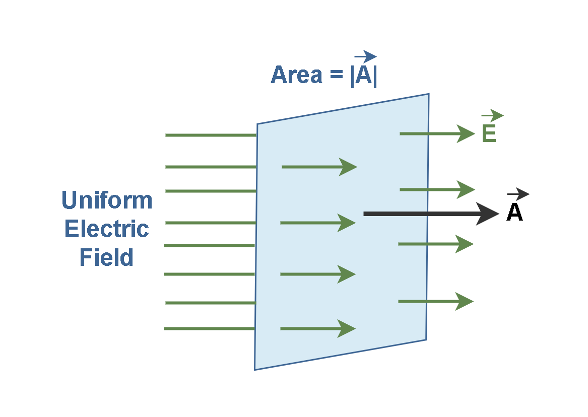
In Figure 1, the number of lines per unit area (N/A) is proportional to the magnitude of the electric field |E|, i.e., |E| ∝ N/|A|. We can rewrite this proportion as N∝|E|.|A|, which means that the number of field lines is proportional to the dot product of E and A. This number is called the electric flux and is generally represented by the symbol Φ_E  in Equation 1.

Then, electric flux is calculated by a dot product of the electric field and the area normal vector. It is a scalar measure of the flow of electric field lines through an area A oriented perpendicular to the field. Note that ϕ_E has SI units of Newton-square meters per Coulomb (N.m²/C)  and also another unit for electric flux is Volt-meter (V.m). It is called electric flux by analogy with the term flux in fluid flow.

In some cases, the surface under consideration ‘A’ might not be perpendicular to the field E, as depicted in Figure 2.

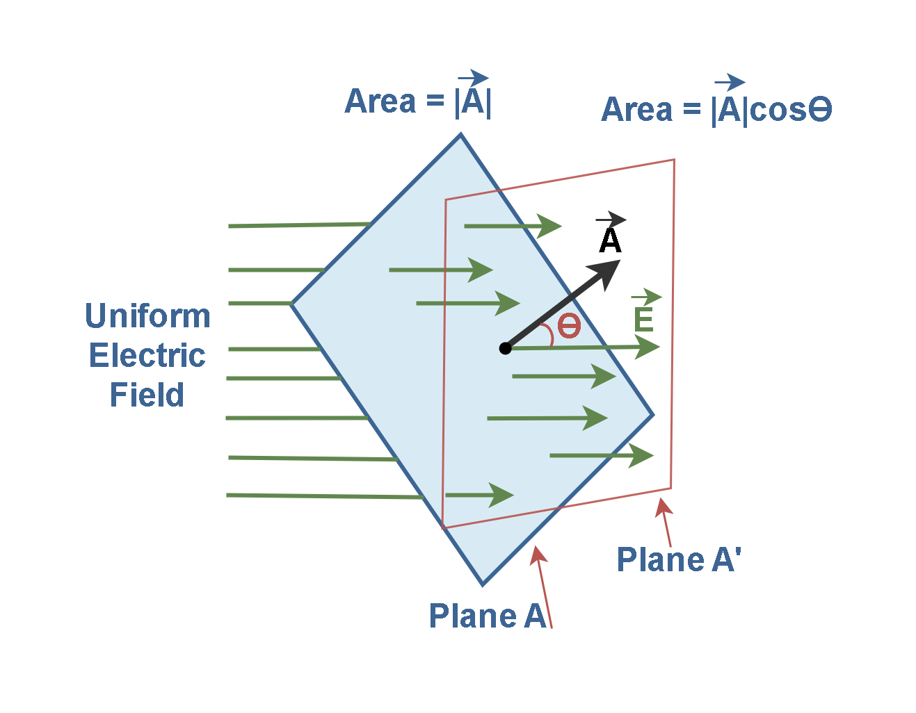
In this position, the normal vector A is at an angle Ɵ in respect to the field E lines. We can define a surface with area A’ which is the projection of A and perpendicular to the field E. Based on trigonometric relations, the projection of one area (A) on another area (A’) comes out by multiplying the first area by the Cosine function of the angle between them. Then, the two areas are related by A’ = A cos Ө. Now, we can say the number of lines that cross the area A is equal to the number of ones that cross the projected area A’.

Thus, the expression of the total electric flux for the uniform field E and the flat surface A is explained in Equation 2.

From Figure 2 and Equation 2, we can conclude that the flux through a surface of fixed area A has the maximum value when the surface is perpendicular to the field (Ө = 0°) and has the minimum value of zero when the surface is parallel to the field (Ө = 90°).

In general, a surface might not be flat, and the electric field may not be uniform (either in magnitude or direction) over the surface. In practice, to find the net flux ϕ_E through the surface, we can divide up the surface into small sections (square patches) with small areas ∆A (as shown in Figure 3). That could be a good approximation to treat them as the electric field E is reasonably constant in this small area.

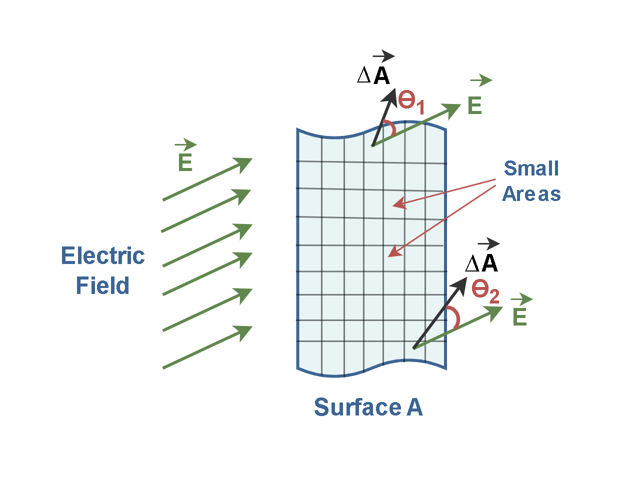
Then, we find the partial flux at every patch and then add up the results (with the algebraic signs included) to get the net flux, as described by Equation 3.

However, for non-geometric shapes or closed surfaces, because we do not want to sum hundreds (or more) of partial flux values, we transform the summation into an integral by shrinking the patches from small squares with area ∆A to smaller partial area elements dA. Each infinitesimal element of area dA has a normal direction to its partial area. We use these small area elements as the variables of integration. The total flux then can be calculated by integrating the dot product of two vectors (E . dA) over the total surface, as described by Equation 4.

Where the electric field is uniform and the surface is flat, the quantity |E| or the product (|E|. cos Ө) is a constant and comes outside the integral. The remaining ∫dA is just an instruction to sum the areas of all the partial elements to get the total area. Note that flux is still a scalar quantity. The small circle on the integral sign indicates that we must integrate over the entire surface, to get the net flux through a closed surface.

In this subject, we are only interested in finding the flux for a special class of surfaces, ones which we call Gaussian surfaces. Such a surface is a closed surface that is, it encloses a particular volume of space and doesn’t have any holes in it. This imaginary surface is used strictly for mathematical calculation, and need not be an actual or physical surface.

The Gaussian surface has a shape determined by the symmetry of the charge distribution. This imaginary surface is chosen so that the electric field is constant everywhere on it. The Gaussian surface can vary in shape and size. It is a closed surface that has an inside and an outside: an example is a sphere.

Figure 4 shows a Gaussian surface in the form of a closed cylinder. It lies in a uniform electric field E with the cylinder’s central axis (along the length of the cylinder) parallel to the field. Then, flux might enter on one side and leave on another side.

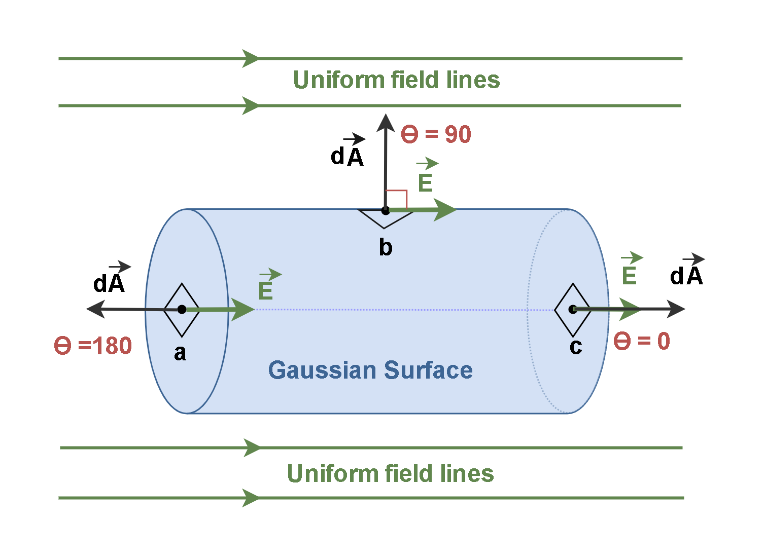
We can find the net flux Φ_E with Equation 4 by integrating the dot product (E.dA) over the cylinder’s surface. Recall that this term is converted to (|E|.|dA|.cosӨ) in the calculation. To simplify calculations, we can break up the entire surface into three sections with which we can actually evaluate an integral. Three terms of integration are integrals over the left cylinder cap (section a), the curved cylindrical surface (section b), and the right cap (section c). Equation 5 explains the calculation procedure.

By convention, for a closed surface, the flux lines passing into the interior of the volume are negative and those passing out of the interior of the volume are positive. This convention is equivalent to requiring the normal vector of the surface to point outward when computing the flux through a closed surface. It means the angle Ө between the normal vector and the electric field lines determines the algebraic sign of each term in the calculation. In this way, in section ‘a’ the angle Ө = 180° (then cos Ө = -1), and in section ‘b’ we have Ө = 90° (cos Ө = 0), and for section ‘c’ the angle Ө = 0° (cos Ө = 1).

Let the total area of sections ‘a’ and ‘c’ be A. Substituting the results into Equation 5 leads us to: Φ_E  = -EA + 0 + EA = 0.

Therefore, the net flux is zero because the field lines that represent the electric field all pass entirely through this Gaussian surface, from the left to the right. It means that there is no charge as the source of the electric field inside the Gaussian cylinder.

Gauss’s Law

Gauss’s law, also known as Gauss’s flux theorem, was developed by the mathematician Karl Friedrich Gauss (1777–1855). It is essentially a technique for calculating the electric field on a closed surface, called a Gaussian surface. Gauss’s law relates the electric flux through a closed surface and the total charge inside that surface.

Consider a point charge q surrounded by a spherical Gaussian surface of radius R centered on the charge, as in Figure 5.

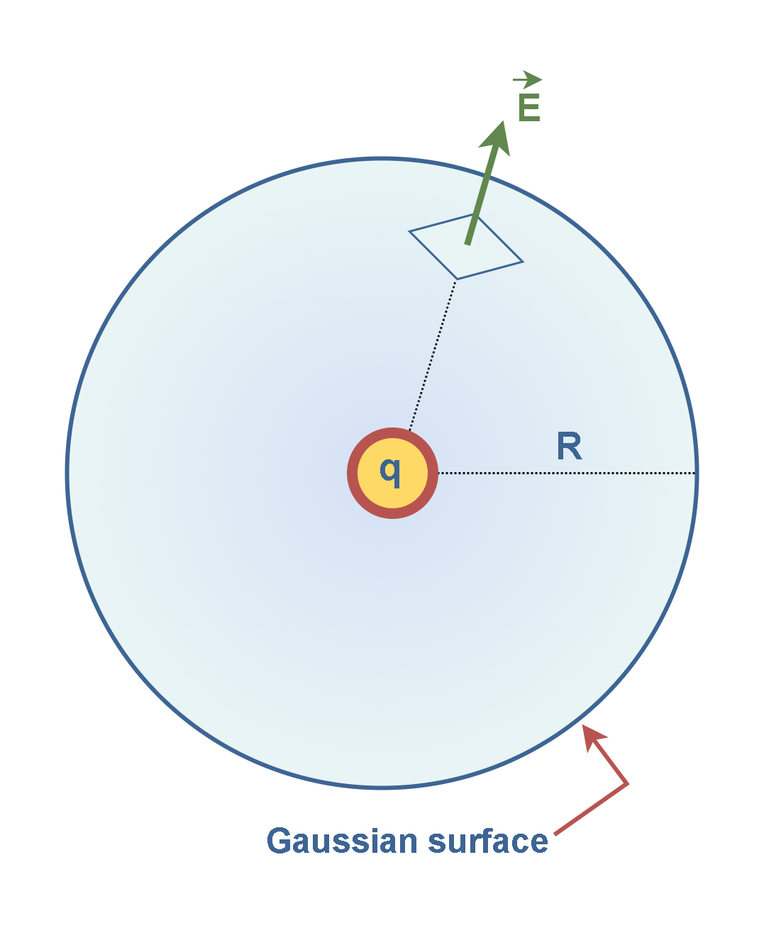
As we mentioned in previous articles, the magnitude of the electric field everywhere on the surface of the sphere with radius r is calculated by Equation 6.

The constant ε₀ is called the permittivity of free space and has the value: ε₀ = 8.85 x 10^-12 C²/N.m²

Note that the electric field is perpendicular to the spherical surface at all points on the surface. Therefore, the electric flux through the closed spherical surface that surrounds the charge q is (|E|.|A|), where A = 4πR² is the entire surface area of the sphere. Equation 7 calculates the electric flux.

Equation 8 gives us the final result:

This result says that the electric flux through a sphere that surrounds a charge q is equal to the charge magnitude divided by the constant ε₀. This result can be proven for any arbitrary closed surface that surrounds the charge q.

Suppose we choose a closed surface A in some environment where there are charges and electric fields. We can compute the electric flux Φ_E  on A. We can also find the total electric charge enclosed by surface A, which we will call Q_inside. This leads to the following general result, known as Gauss’s law: ” The electric flux Φ_E through any closed surface is equal to the net charge inside the surface, Q_inside, divided by ε₀“. Equation 9 explains the theorem in mathematical form.

Gauss’s law uses only the component of the electric field that is normal (perpendicular) to the Gaussian surface. This component is mostly denoted by E_n. In other words, Gauss’s law states that the integral of the normal component of the electric field over any closed surface is proportional to the net charge contained inside that surface.

Equations 6 – 9 hold only when the net charge is located in a vacuum or in air (which are the same for most practical purposes). In all the Equations, the net charge Q_inside is the algebraic sum of all the enclosed positive and negative charges, and it can be positive, negative, or zero. We include the sign, rather than just use the magnitude of the enclosed charge because the sign tells us something about the net flux through the Gaussian surface: If Q_inside is positive, the net flux is outward; if Q_inside is negative, the net flux is inward.

The exact form and location of the charges inside the Gaussian surface are also of no concern. The only things that matter on the right side of Equations 6 – 9 are the magnitude and sign of the net enclosed charge. The electric field due to a charge outside the Gaussian surface contributes zero net flux through the surface, because as many field lines due to that charge enter the Gaussian surface as leave it.

Usefulness Of Gauss’s Law

Gauss’s Law is a fundamental principle in electromagnetic theory and it also has several applications in electromagnetism. Gauss’s law is equivalent to Coulomb’s law (which we have already explained in previous articles). But, while Coulomb’s law is formulated in terms of point charges, Gauss’s law is formulated in terms of continuous charge distributions. In such special cases, Gauss’s law is far easier to apply than Coulomb’s law.

We can use Gauss’s Law to find the electric field around charge distributions that have some type of symmetry, but we need to choose Gaussian surfaces of different shapes to take advantage of the symmetry.

There are mostly three kinds of symmetry that work:

• Cylindrical symmetry: In cases of line or cylindrical charge distributions, we can make our Gaussian surface a cylinder (see Figure 4, where the charge can be distributed along the axis of the cylinder or over a cylindrical surface inside the blue Gaussian cylinder).
• Spherical symmetry: In cases of point charges or spherical distributions, we can make our Gaussian surface a concentric sphere (see Figure 5).
• Planar symmetry: In planar charge distributions, we can make a Gaussian “pillbox” that straddles the surface (see Figure 6).

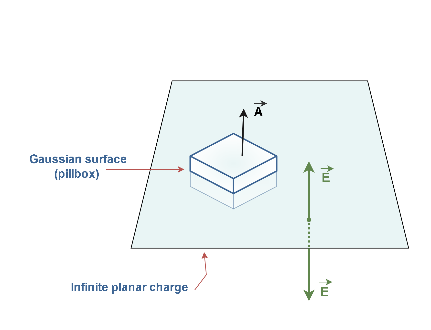
Figure 6 demonstrates how Gauss’s law can be applied to determine the electric field strength around an infinite planar charge distribution. In Figure 6, the large flat surface represents an infinite plane of uniform charge. A small box-like shape is the Gaussian surface. Green arrows indicate that the electric field is perpendicular to the plane and equal in magnitude on both sides, but opposite in direction. A black arrow points upward from the top of the pillbox, representing the area vector of the Gaussian surface.

Although cases (2) and (3) technically require infinitely long cylinders and planes extending to infinity, we shall often use them to get approximate answers for “long” cylinders or “large” planes, at points far from the edges.

Finally, even when the charges are not symmetrically distributed, Gauss’s law can still be used to give a rough estimate for design exploration or for checking the result from a computer program.

Summary

• The amount of electric field passing through an area oriented perpendicular to the field is defined as the electric flux, Φ_E.
• Φ_E has SI units of N·m²/C (Newton-square meters per Coulomb).
• The normal vector with a magnitude equal to the area of a surface indicates the surface position relative to the field lines.
• Charges can be surrounded by an imaginary surface, called a Gaussian surface.
• Gauss’s law states that the electric flux through a closed surface (a Gaussian surface) is proportional to the charge contained inside the surface.
• An inward penetrating field produces negative flux. An outward penetrating field produces positive flux. A field parallel to the surface (skimming) produces zero flux.
• Charge outside the Gaussian surface, regardless of its magnitude or proximity, is not included in Gauss’s law calculations.
• The field of a uniformly charged spherical surface is identical to that of a point charge located at the center of the sphere with the same total charge.
• Gauss’s law may be an easier alternative to Coulomb’s law in some applications.
• Gauss’s law combined with symmetry arguments may be sufficient to determine the electric field due to a charge distribution.

Please follow and like us: