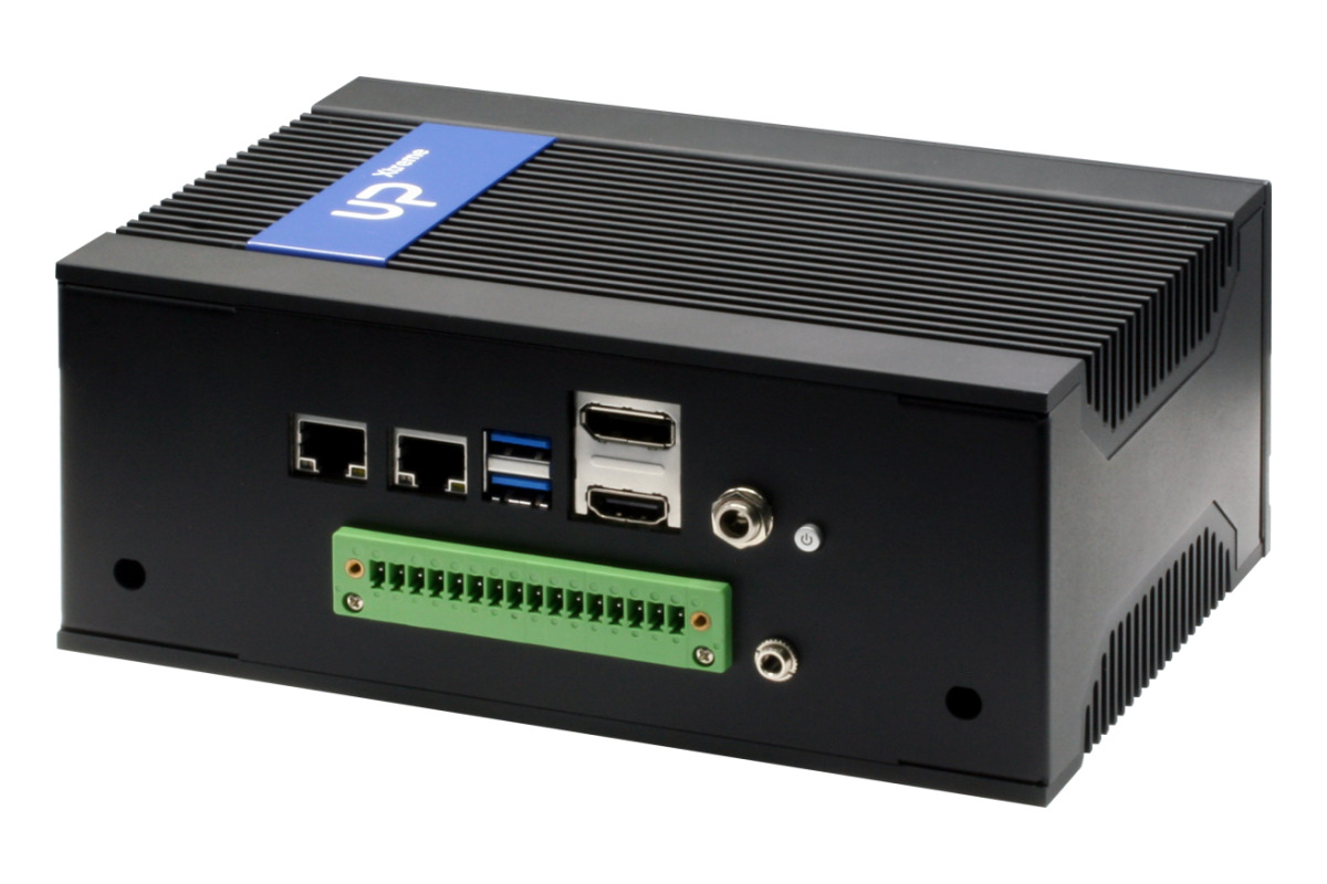
Many developers and users of security solutions are looking for ways to get more out of their surveillance systems by deploying intelligent edge computing platforms. UP Xtreme, from AAEON’s UP Board division, is being deployed along with technology from partners including Intel®, Milestone and SAIMOS® to bring Smart Surveillance to these customers with the UP Xtreme Smart Surveillance kit.
With the ever-increasing importance of on-site security, surveillance cameras are installed virtually everywhere, recording footage passively. Smart surveillance takes things to the next level by adding intelligent processing of data that’s already being gathered to analyze traffic with heatmaps, monitor areas with virtual fences, or reacting to data in other ways to allow for automated control or alerting staff on premises. UP Xtreme Smart Surveillance provides all the technology needed to power these applications in one box, working as an AI-enabled NVR solution to proactively monitor video streams supporting up to 32 cameras simultaneously (Intel® Core™ i7 model with Milestone XProtect® Express+).
Working with technology partners Intel, Milestone, and SAIMOS, AAEON’s UP team is deploying the UP Xtreme Smart Surveillance solution to overcome the challenges present in traditional security camera systems. UP Xtreme Smart Surveillance works by integrating video management software (VMS) from Milestone with video analytic software from SAIMOS, then adding a deep learning AI edge inference through the Intel® Distribution of OpenVINO™ toolkit, to provide a total package solution that saves deployment time and cost for end users, as well as overcoming challenges such as storage issues. The AI inference is also accelerated with two Intel® Movidius® Myriad™ X VPUs, helping provide even more power alongside the 8th Generation Intel® Core™ processor that comes with the UP Xtreme system.
“UP Xtreme Smart Surveillance offers video analytics combined with a modern video management system, integrating everything into a one-box solutions which can be deployed with both new or existing infrastructure,” said Jürgen Konetschnig, CTO of SAIMOS.
“The hardware and software are integrated to make deployment of smart surveillance applications easier and simpler for users in any field,” Jügen added.
The BOXER-8130AI is built to easily integrate into any environment. Featuring six MIPI CSI-2 interfaces, the BOXER-8130AI can support up to six MIPI cameras. The BOXER-8130AI is also built for easy maintenance, with an SD Card slot, USB OTG, remote ON/OFF and almost all of its I/O ports together on one side. The BOXER-8130AI also features two antenna ports, perfect for mobile or AIoT gateway applications.
Once UP Xtreme Smart Surveillance is installed, the platform is easy to use and provides intuitive analytic parameter settings for users to have a comprehensive overview of the entire surveillance installation. UP Xtreme Smart Surveillance provides key functions to support applications such as people/object counting, heatmapping, virtual fence and perimeter protection, dynamic blurring and object detection. The system uses data analytics and edge computing to provide real time analysis, and can provide proactive measures through alerting relevant staff as soon as an incident is detected.
UP Xtreme Smart Surveillance also provides users with a solution that is flexible and scalable from number of cameras to AI acceleration. UP Xtreme Smart Surveillance is helping to bridge the gap for modern security and surveillance systems. UP Xtreme Smart Surveillance is available through the UP Shop website or by contacting AAEON and UP Team representatives.
Loren Browman, a security analyst recently published a guide to automated unlocking of Nordic Semiconductor’s nRF51-series systems-on-chips (SoCs) which claims to be protected, enabling a full memory dump or interactive debugging regardless of protection settings. In a blog piece for security firm Optiv, Loren Browman writes
“Recently, while conducting an assessment for a product based on the nRF51822 System on Chip (SoC), I found my target’s debug interface was locked — standard stuff… Reading up on the nRF51 series SoCs revealed that this is how these chips are designed. It’s always possible to perform a full memory recovery/dump, even if read back protection is enabled.”
He continue:
“I wanted to build on what others have discovered, extending the attack to completely and automatically bypass the memory protection mechanism offered by these SoCs. Beyond reading memory, I also wanted to unlock the device to support interactive debug sessions with my target.”
This resulted to nrfsec, which is an open source research security tool published under the GNU General Public License 3, used for unlocking and reading memory on nrf51 series SoCs from Nordic Semiconductor.
Features of the nrfsec includes:
Read all target memory, bypassing the Memory Protection Unit (MPU) settings with integrated read gadget searching.
Automated unlock feature: read all program and UICR memory, erase all memory, patch UICR image, reflash target into unlocked state.
Boot delay command flag for interacting with target prior to performing memory read, allowing for RAM dumps.
All firmware images are saved for importing into your favorite disassembler.
About nrfsec, Loren Browman says
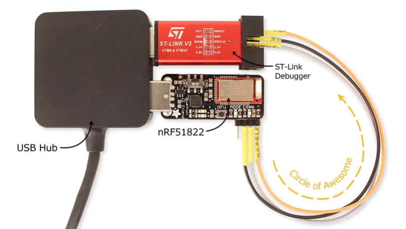
“[nrfsec] can automate the entire outlined process for you… Letting you uncover the internal working of any nRF51 based product.” Once it is unlocked, the tool establishes a debug session to the now-unprotected SoC. For installation, nrfsec is built on the pyswd library and currently only works with the ST-Linkdebugging interface.
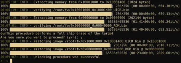
nrfsec requires python 3.7+ to run and can be installed with pip. For nrfsec to work, it will first of all make a quick info check to ensure that nrfsec is able to communicate with both the debugger and the target. The output for the info will also specify if the target is currently locked with some additional interesting target information. Then nrfsec will automatically find a useable read gadget and dump all memory on a locked target. If the target is not already locked, you can issue the lock sub-command, and it will lock the again. If you want to unlock the target, you issue the unlock sub command which will perform the following steps:
Read all memory regions (most importantly, ROM and UICR) and save the images.
Perform a full target erase, this will enable writing to the UICR again.
Patch the UICR image extracted during step 1 to disable read back protection.
Re-flash the ROM and patched UICR back to the target.
More details of how the tool works and how to use it can be found on the Optiv blog, while nrfsec itself is available to download from GitHub, or can be installed from the pip Python package manager.
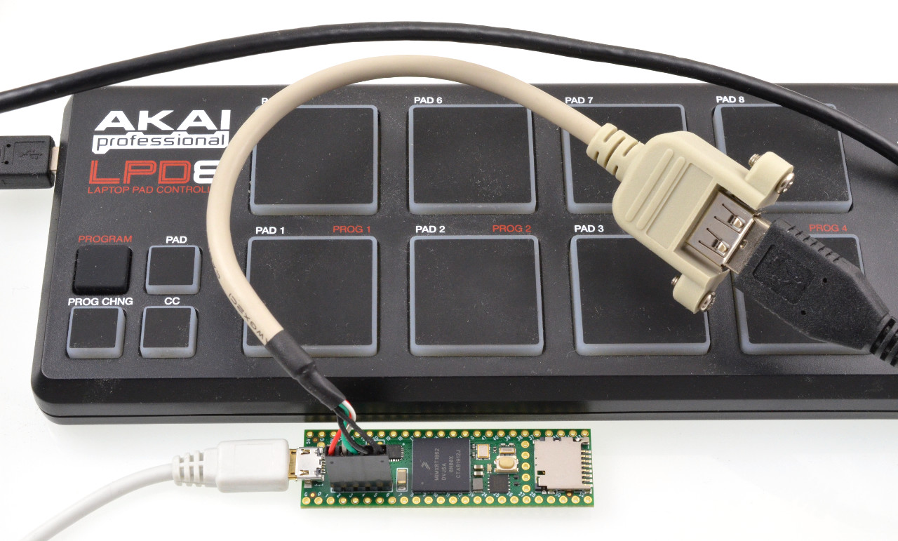
Teensy is another line of microcontroller boards designed to offer maximum I/O capabilities backed up by fully featured software libraries to run on Arduino. Loved by makers around the world for a number of reasons, these Arduino compatible boards have proven to be an astounding development platform in a small form capable of implementing many types of projects. They are usually built around high-performance 32-bit ARM chips that offer faster clock speeds, expanded set of hardware peripherals, and extended serial communication ports.
Just like other popular platforms, Teensy development boards have gone through many iterations each with different computing power, pins, and performance specifications. Just last year, the Teensy 4.0 priced at $19.95 was released, and now v 4.1, an update of the already mighty 4.0 has been added to the league.
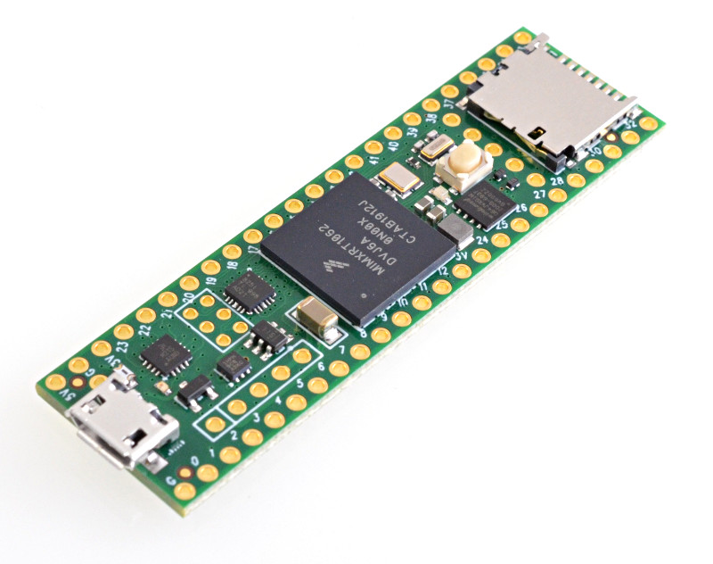
One big addition to the newly released Teensy 4.1 is the fast Ethernet to support low latency and high bandwidth applications. It is a bigger size than the 4.0 but adds more peripherals, memory, and GPIOs. PJRC, however, says that both Teensy 4.1 and 4.0 serve different segments of the market, so one is not a replacement for the other.
“Not every project requires so much or extra memory. Teensy 4.0 fills those needs. But when you do need more I/O, more memory, fast Ethernet, or connecting USB devices or fast SD card access, the larger Teensy 4.1 brings this extra I/O capability to a platform designed for real-time use with fast 600 MHz M7 performance.”
Highlight features of the Teensy 4.1 include:
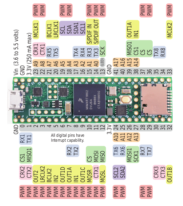
NXP i.MX RT1062 Arm Cortex-m7 processor running at 600 MHz
8MB Flash storage and 1024 KB RAM
MicroSD socket and footprints for 2x extra QSPI chips plus program memory
1x micro USB port for power and programming
6-pin Ethernet header via 10/100 Mbit DP83825 PHY for networking
2x USB ports of 480 MBit/sec
2x I2S and 1x S/PDIF Digital Audio
1x SDIO native SD (4 bit)
35x PWM pins, 40x digital pins, 18x analog pins, 8 serial ports and 2x ADCs on chip
3x SPI, 3x I2C
5V Power supply via USB port
Cryptographic Acceleration and Random Number Generator
Dimension: 7.2 x 4.8 cm
More details on the Teensy 4.1 can be found on PJRC news page or the product page where it sells for $26.95. The Ethernet adapter is also available as a DIY project on the 4.1 Ethernet project link.
Sensor boards are manufactured to provide engineers with the ideal platform for developing projects and designs that detect or measure temperature, pressure, humidity, color, motion, and even physical location. They offer necessary support circuitry that allows for the full utilization of sensors for demonstration and evaluation.
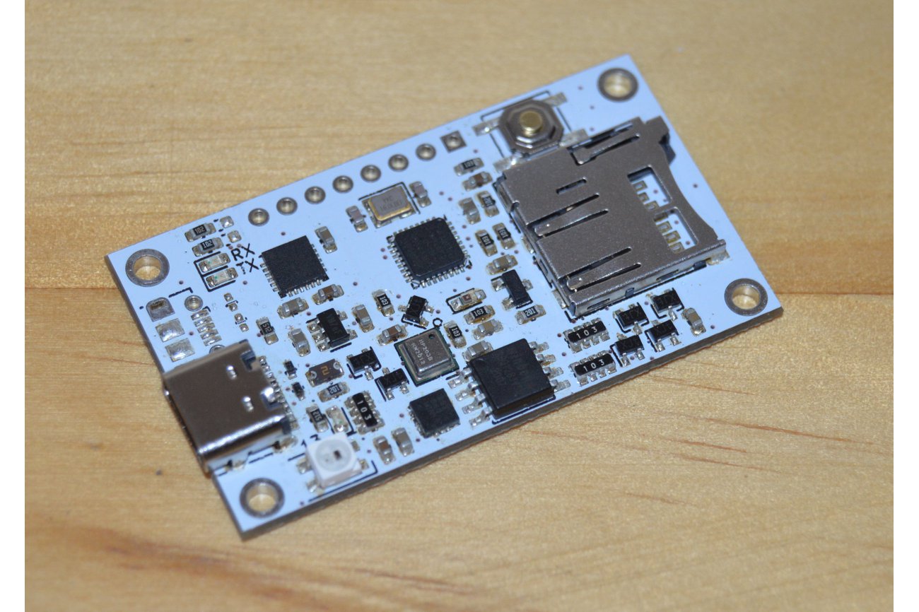
While there’s been a wide range of available sensor development boards from different integrated circuit device manufacturers, the new customizable sensor board by the Bellingham-based company was designed to reduce cost with only desired specifications to be built in at the time of its manufacture. The sensor board integrates a variety of sensors and memory directly onto the board instead of simply breaking out the processor’s pins, thus providing an extremely compact platform to work with. It is cost-effective compared with mass-manufactured breakout boards as it allows you to use a single PCB for every sub-system.
The compatible sensor board is fully compatible with Arduino IDE and comes flashed with Arduino Pro / Pro mini bootloader.
Features and specifications include:
An ATmega328p microcontroller clocked at 16MHz by an external crystal and runs at 5V (standard).
A 16 MB SPI flash chip for storing a moderately large number of sensor readings (optional). The chip memory might be smaller than the usual microSD card, but sufficient for many applications. The flash chip also offers lower power consumption as well as lower code overhead than a memory card.
A USB type-C for USB programming (standard).
A MicroSD card socket for storing large amounts of data that can easily be read off the board (optional).
Serial WS2812B RGB LED (optional)
An HP203b barometer can directly measure both the temperature and pressure of the working environment and calculate the altitudes based on the readings obtained. (optional)
An MMA845Q accelerometer that communicates over 12C (optional).
A temperature sensor that outputs analog voltage depending on the temperature (optional).
A Visible light phototransistor sensor for measuring ambient light (optional)
Up to 6 GPIO pins for expansion along with 5V and ground (optional)
Board’s Dimension: 28 mm x 48 mm (1.1 x 1.8 inch)
The project’s GitHub page has more information on the sensor board including a list of tested and recommended libraries, schematics, and datasheets for each component. Further details can also be found on tindie where the board is currently being sold for $17.99.
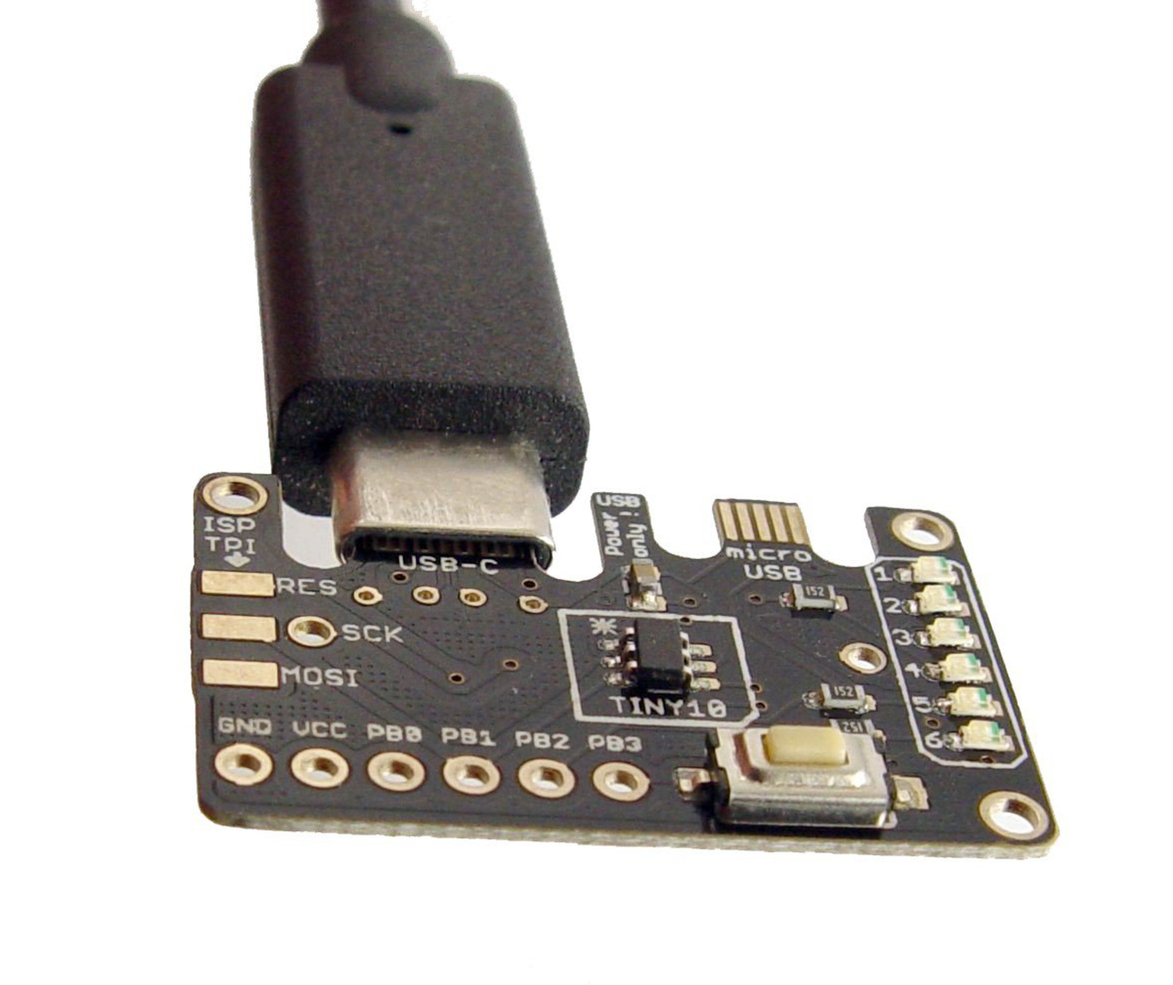
If you like using the simplest possible chip for each of your applications, then the ATtiny10 development board will strongly appeal to you.
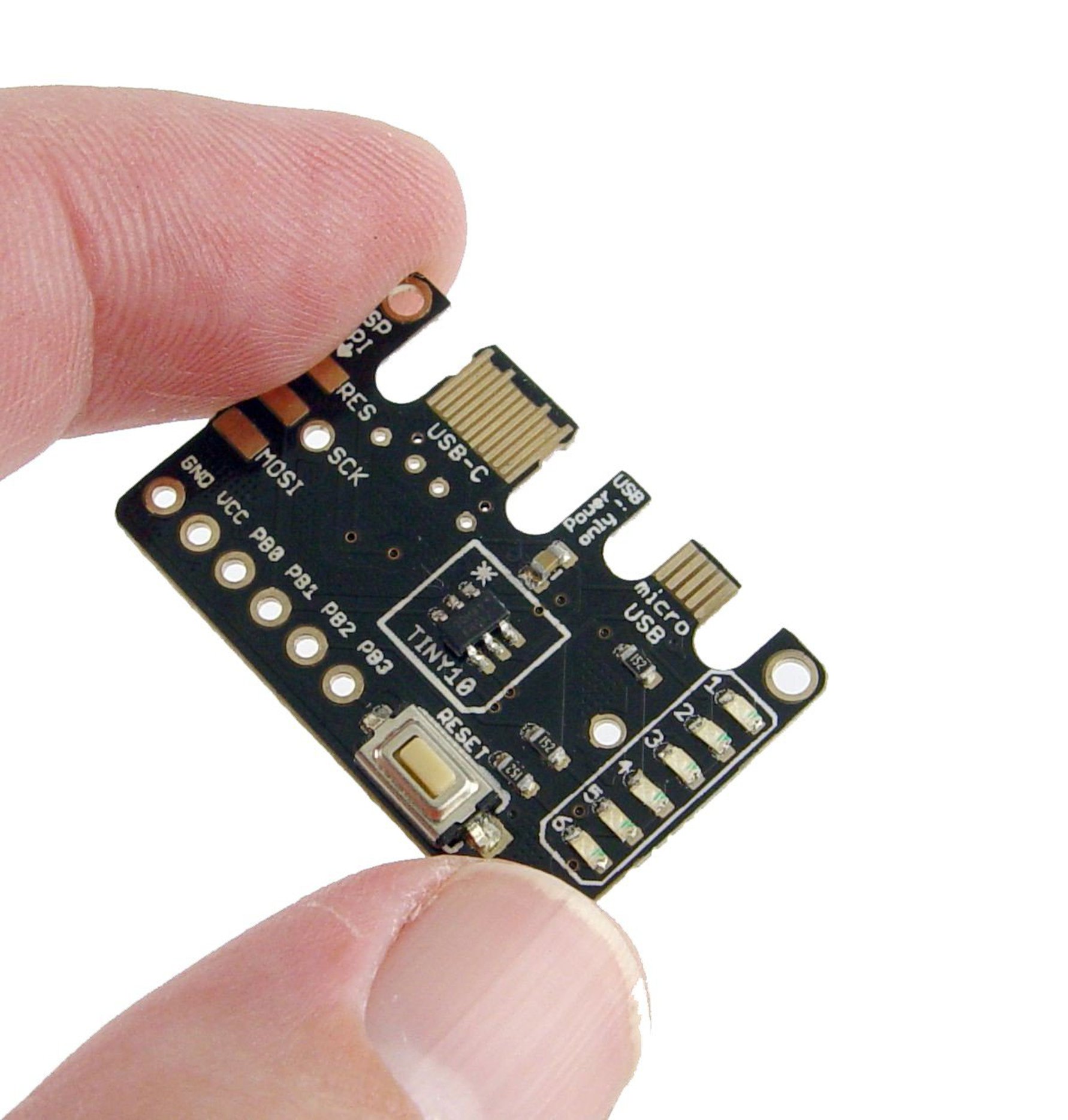
The ATtiny10 development board from Bobricius is a low-power high-performance 6-pin processor equipped with both USB-C and Micro-USB for powering purposes only. True to its name “tiny”, the chip is about the same size as an 0805 SMD resistor but despite its size, the ATtiny10 development board still has features similar to larger AVR chips; still a great way to jump into microcontroller electronics.
The New ATtiny 10 Development Board
“This board is for advanced users”
, says the Slovakia-based designer,
“the ATtiny10 is a high-performance, low-power Microchip 8-bit AVR RISC-based microcontroller that combines 1KB ISP flash memory, 32B SRAM, four general-purpose I/O lines, 16 general purpose working registers, a 16-bit timer/counter with two PWM channels, internal and external interrupts, programmable watchdog timer with internal oscillator, an internal calibrated oscillator, a 4-channel / 8-bit A/D converter, and four software selectable power saving modes,” he adds.
Some features of the new development board include;
Power Options: Either from the header, PCB micro USB, PCB USB-C or CR2032
The Microchip’s miniature 6-pin processor has already been used for quite a number of projects, like the ATtiny10 Thermometer and ATtiny10 POV Pendant. With a host of shields to extend its functionalities, the ATtiny10 development board is considered perfect for designing interface logic for projects and building small gadgets and wearables.
To work with the ATtiny10 on a breadboard, you can make use of an SOT23 breakout board, just like the one available from Sparkfun.
The ATtiny10 development board comes preloaded with sample flashing codes, more information on the board can be found on Tindie where it currently sells for $12.99.
Technoblogy also has further details about the ATtiny10 including simple applications with example programs and step by step instructions on how to program the board using the familiar Arduino IDE. Shipping usually takes about 2 – 3 days but Bobricius says that things may become different now as a result of the current pandemic.
There’s many a time when you want to connect a white LED to a microcontroller operating from a 3 V supply voltage. Unfortunately, this doesn’t work and your nice white LED only lights up feebly or not at all.
Why does it work perfectly with red and green LEDs, but not with white? A bit of data sheet research reveals the reason: white LEDs have a forward voltage of 3.2 V, so a 3 V supply is simply not enough to let them light up properly. The advice you often see in online forums is to use a boost converter to generate a higher voltage, along with a transistor switch to control the LED. For just a single LED, this seems like a lot of overhead.
The good news is that there’s an easier way. And it only needs one inexpensive component: an inductor, which costs next to nothing. If you wire it up right and drive it the right way, your white LED will light up nicely — and this even works with a microcontroller supply voltage as low as 2.5 V. Magic? Not at all.
Elektor Article: LED Booster for Microcontrollers – [Link]
The fundamental relation between the current, voltage, and resistance is known as Ohm’s law and is probably the most famous and elementary physical law of electronics. It is in 1827 when the German physicist Georg Simon Ohm publishes for the first time in the book “Die galvanische Kette, mathematisch bearbeitet” (in English: The mathematical study of the galvanic circuit) an early form of the law that will later take his name.
In the first section we will present the macroscopic Ohm’s law which is the form that is shown to students early in the learning process.
In the second section, we will see that different forms of the equation can be adapted depending on the topology of the circuit and the nature of its source, in particular when considering the AC regime.
More advanced concepts are presented in the third section where we focus on the mesoscopic definition of the equation which is known as the local expression of Ohm’s law.
Presentation
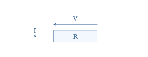
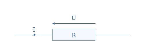
We consider an electric current I, flowing through a resistor R which produces a potential difference U at its terminals:
fig 1: Current crossing a resistor presenting a voltage at its terminals
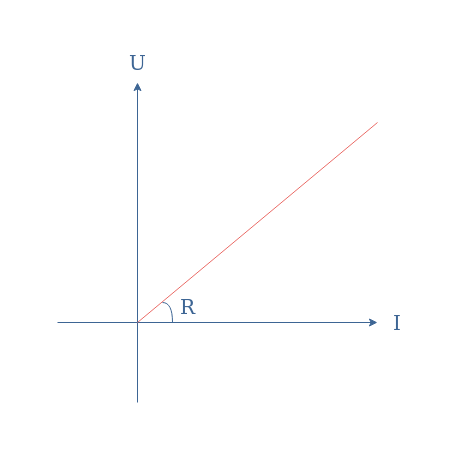
Ohm’s law establishes a simple linear relation between these three parameters such as U=R×I. Any electrical component that verifies Ohm’s law can be labeled as an ohmic conductor and presents a voltage-current characteristic such as presented in Figure 2:
fig 2: U/I Characteristic of an ohmic conductor
It is important to note that Ohm’s law is empirical, meaning that it comes from experimental observations and not from a theory.
The macroscopic form is widely used in electronic circuits and it is a very useful formula to know. We can compute an unknown parameter (R for example) with the knowledge of two others parameters (U and I for example). Moreover, it allows us to write the expression of the dissipated power in a resistor under the form P=R×I2.
Equivalence in AC regime
Ohm’s law can be generalized when the current and voltage are sine waveforms. In this case, we use the complex notation to write the law such as U=Z×I with Z being the complex impedance of a set of linear components (resistor, capacitor, and inductor).
In resistor
If we consider again the circuit presented in Figure 1 in AC regime, Ohm’s law can be written such as u(t)=Ri(t) with i(t)=I×sin(ωt), u(t)=U×sin(ωt+φ), and I, U being the amplitudes of the respective signals. However, since the phase difference in a purely resistive component is equal to zero, we obtain U=RI.
In the AC regime, the expression of Ohm’s law in a resistor is similar to in the DC regime.
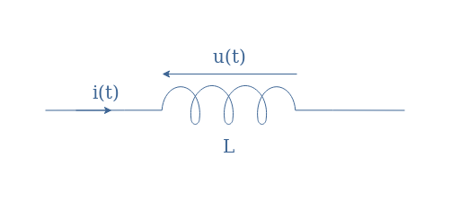
In inductor
Things get a little different when considering reactive elements, let’s begin with the inductor:
fig 3: AC voltage and current across an inductor of inductance L
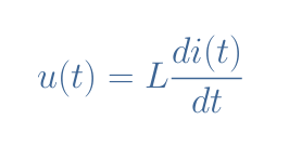
According to Lenz’s law, the voltage u(t) produced by an inductor is proportional to both the inductance and the variations of the current i(t) as shown in Equation 1:
eq 1: Relation between the voltage and current in an inductor
It can be shown from Equation 1 the relation between current and voltage can be written u(t)=Lω×Isin(ωt+φ). The demonstration is even easier when using the complex notation and knowing that the derivation operation in the complex domain is similar to multiplication by jω which consists in multiplying the phasor i(t) by ω and proceeding to a rotation of φ=+π/2 rad (see the tutorial about Phasors Diagrams & Algebra).
In an inductor, the current and voltage signals are therefore phase-shifted of Δφ=+π/2 rad. Since the voltage is usually considered to be the reference, its expression remains unchanged (u(t)=U×sin(ωt)), while the current can be written i(t)=I×sin(ωt+φ).
Ohm’s law in an inductor can be written U=LωI ; φ=+π/2 rad.
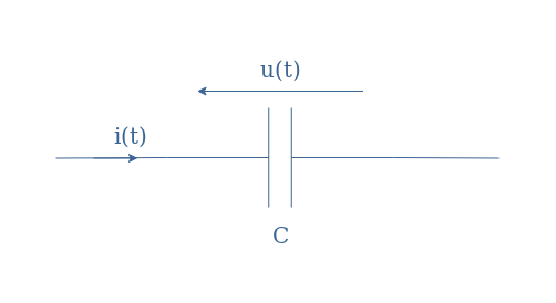
In capacitor
Finally, we consider a capacitor in the AC regime:
fig 4: AC voltage and current across a capacitor of capacitance C
In this configuration, the charge of the capacitor is a function of time and its expression is q(t)=C×u(t). Since i(t)=dq(t)/dt, we can demonstrate directly or by using the complex notation that i(t)=-Cω×Usin(ωt+φ).
If we consider again the voltage to be the reference signal, the phase-shift is here Δφ=-π/2 rad, the expression of the current is, therefore, i(t)=I×sin(ωt-φ).
Ohm’s law in a capacitor can be written U=I/Cω ; φ=-π/2 rad.
Local form
In this section, we discuss a more advanced concept known as the local form of Ohm’s law. Prior to presenting this special form, we need to introduce and define some concepts. We want to note that in the following, the vectors are bolded while the scalars are not.
Presentation and definitions
The local form can be applied to an intermediary scale of space between microscopic and macroscopic known as the mesoscopic scale. Typically, the mesoscopic scale is considered to be large enough to contain a large number of particles in an elementary volume (electrons in our case) but small enough so that the parameters such as the pressure and temperature stay local.
We usually refer to the electrons as “charge carriers” or simply “carriers”, they are defined by the carrier density ne, their speed vector v, the elementary charge e, and their mass me.
From these parameters, we can define an important vector j known as the current density to be j=-enev. The term -ene is also known as the charge density and noted ρe.
Drude model
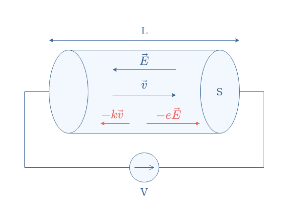
Consider an ohmic conductor of section S submitted to a certain voltage V, this potential difference induces an electric field E which forces the carrier of the conductor to move:
fig 5: Schematic view the forces (in red) and fields inside an ohmic conductor
The movement of the carriers is dictated by two forces that act in opposite directions:
The electrical force -eE tends to move the electrons in the opposite direction to the electrical field (same direction for positively charged carriers).
A friction force -kv that tends to slow down electrons. This force is due to the motionless charges that constitute the crystal lattice of the ohmic conductor, which the electrons have a certain probability to crash in. The parameter k is a constant that depends on the material considered to be the conductor.
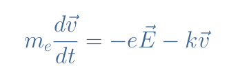
The Drude model (1900) consists of taking into account these two forces and apply the second law of Newton to the carriers:
eq 2: Newton’s second law in the Drude model
Expression of the local form
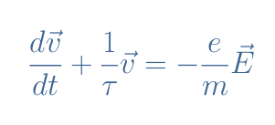
We can rearrange Equation 2 and write k/m=1/τ with τ being the relaxation time parameter of the ohmic conductor:
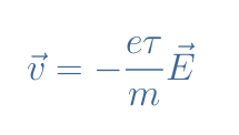
In permanent regime (t>>τ), this first-order differential equation accepts the following expression as a solution:
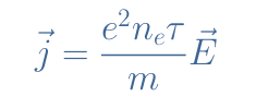
Finally, the current density can, therefore, be rewritten such as:
We usually write the scalar term σ which is known as the electric conductivity, the local Ohm’s law states that j=σE.
The local form is particularly helpful for studying the electrical properties at a microscopic scale.
Electric resistance and macroscopic Ohm’s law
The electric field in the ohmic conductor can be written E=(V/L)n with n being a unit vector in the same direction as E.
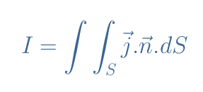
The electric current I is defined as:
The current (C/s) can indeed be understood as the sum of the current density (C/m2/s) taken across the section (m2).
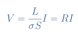
For the topology presented in Figure 5, the previous expression can be simplified to I=σES. When replacing the field E by V/L, we obtain:
Finally, we can conclude that the local form of Ohm’s law enables us to retrieve both the macroscopic Ohm’s law and the definition of the resistance R=L/(σS). We can also note that 1/σ can be replaced by ρ which is defined as the resistivity of the ohmic conductor.
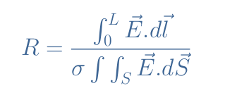
The simplification of the integral expression, however, appeals to two strong hypotheses: the conductivity σ is constant across the material and the current density j is colinear with the axis of the material and uniform. Basically, these two hypotheses can be gathered by assuming that the material is isotropic (uniformity in all orientations).
In the general case, for any topology and if the material is anisotropic, the resistance can be computed with the following formula:
Conclusion
This tutorial has focused on the famous physical law known as Ohm’s law. A recap is given in the first section where its framework, definition, consequences, and uses are shown.
The second section gives a more general form of the law where the supply source works in the AC regime. When considering the three elementary components of electronics, we realize that the form of the law in the AC regime does not change for the resistor but is written differently for the reactive components.
In the final section, we present the local form of Ohm’s law which is adapted for an intermediary scale between the macroscopic and microscopic world: the mesoscopic scale. Many new definitions and concepts are first introduced before explaining through the Drude model how to obtain the local expression. Finally, we demonstrate that the macroscopic form of the law along with the expression of the resistance can be retrieved from the local form.
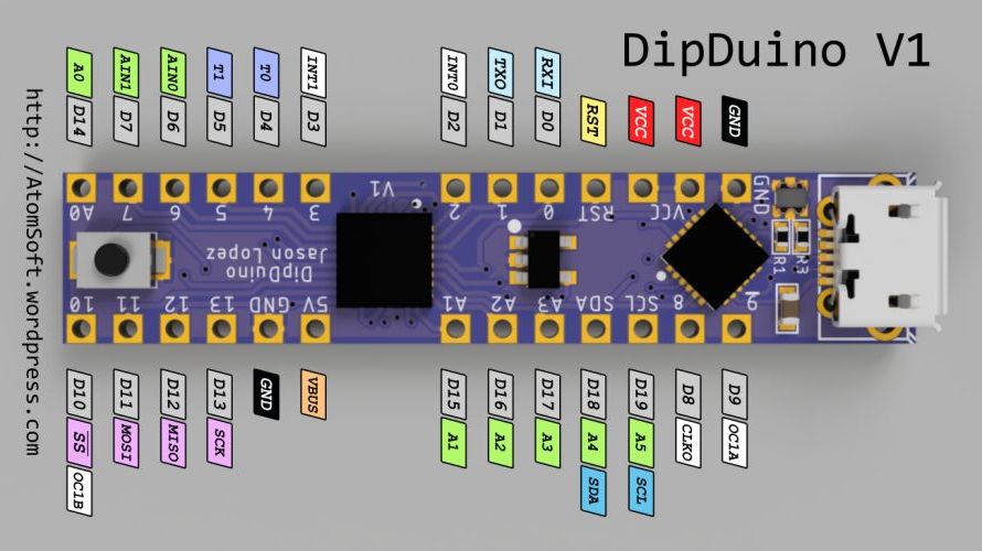
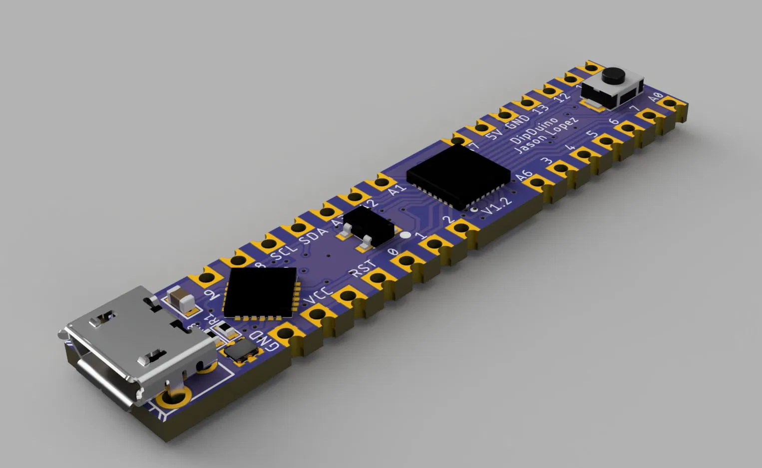
DipDuino is an Arduino in 0.3in DIP form. It runs the Atmega328P. Uses an onboard CP2104 to program itself and comes pre-programmed with Arduino Bootloader. Will act as a Arduino Pro or Pro Mini. Available in Tindie Store.
The DipDuino is a FULL ARDUINO (Minus the A6 & A7 pins). Comes in 5v and 3.3v versions. There is a RGB LED onboard to show the status of Power and UART Transmissions. Green for Power and RED/Blue for Rx/Tx.
Comes with a Reset button on board as well and a LDO for 3.3v Versions. For 5v Versions power is taken straight from USB. Please be safe and careful not to short it.
DipDuino – is an Arduino in 0.3in DIP form – [Link]
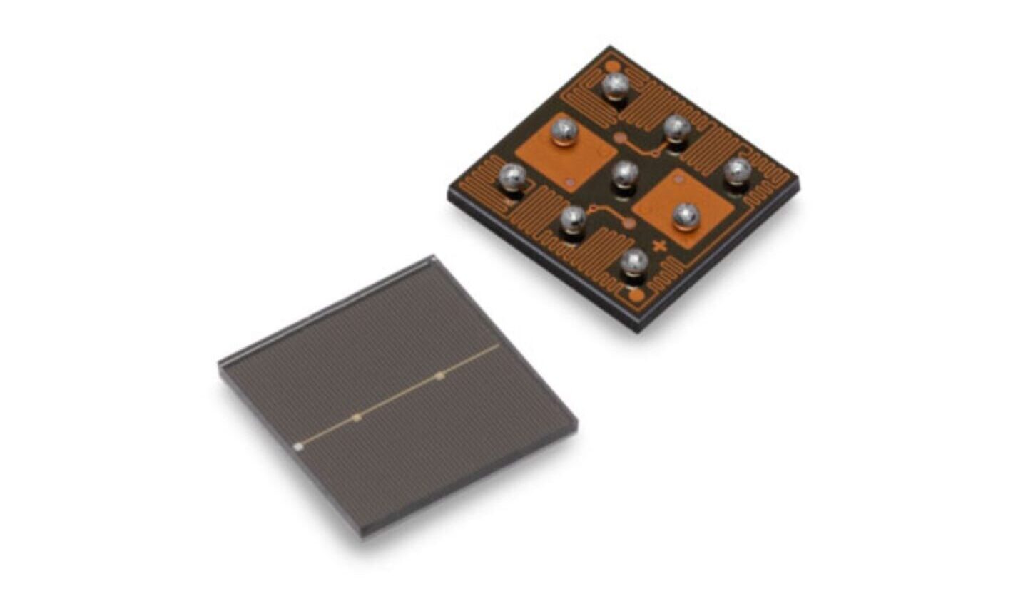
The Broadcom® AFBR-S4N33C013 is a single silicon photomultiplier (SiPM) used for ultra-sensitive precision measurement of single photons. The active area is 3.0 × 3.0 mm2.
The high packing density of the single chips is achieved using through-silicon-via (TSV) technology and a chip-sized package (CSP). Larger areas can be covered by tiling multiple AFBR-S4N33C013 CSPs almost without any edge losses. The protective layer is made by a glass highly transparent down to UV wavelengths, resulting in a broad response in the visible light spectrum with high sensitivity towards blue- and near-UV region of the light spectrum.
The AFBR-S4N33C013 SiPM is best suited for the detection of low-level pulsed light sources, especially for the detection of Cherenkov- or scintillation light from the most common organic (plastic) and inorganic scintillator materials (for example, LSO, LYSO, BGO, NaI, CsI, BaF, LaBr). This product is lead-free and compliant with RoHS.
Key features
High PDE of more than 54% at 420 nm
Chip-sized package (CSP)
Excellent SPTR and CRT
Excellent uniformity of breakdown voltage, 180 mV (3 sigma)
Additional features
Excellent uniformity of gain
With TSV technology (4-side tileable), with high fill factors