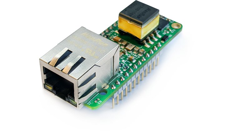
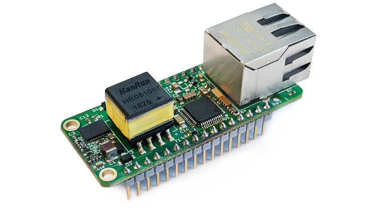
PoE FeatherWing is an Ethernet FeatherWing with 4W of PoE power with globally unique MAC.
Adafruit provides an Ethernet FeatherWing for its popular Feather ecosystem – a valuable option for IoT and automation projects. But it has its limitations. The Feather still needs to be powered separately, and no globally unique MAC address is provided for the user, making deployment hard.
What if we could fix these issues? What if there was a drop-in replacement that would not only provide Ethernet, but also power your Feather, and give you a globally unique MAC? And still be 100% compatible in size, connections and software support? Enter the PoE-FeatherWing!
Features
PoE: Isolated IEEE 802.3at Class 1, Mode A and Mode B Power over Ethernet, with 4 W of output power available.
Globally unique MAC address: A Microchip 24AA02E48 provides a real globally unique MAC address, allowing actual field deployment.
Works with existing software: A WIZnet W5500 Ethernet controller ensures full compatibility with existing software written for the Adafruit Ethernet FeatherWing.
Drop-in replacement: With board size and connections identical to the Adafruit Ethernet FeatherWing, it’s a true drop-in replacement.
Giant Board compatibility: A solder jumper allows for easy compatibility with the Giant Board Feather form-factor Linux SBC, without needing to add a fly wire for the IRQ (interrupt request signal).
The PoE FeatherWing is due to land on Crowd Supply soon; pricing has yet to be confirmed.
This smart device is able to monitor and display CO2, TVOC, PM, temperature, humidity and air pressure measurements. by Roman Novosad
Most of the modern applications focus on measuring outdoor air pollution. This is indeed very important and useful, however most of the time in person’s life is spent indoors. This is also an environment, where one is able to influence the climate using various air purifying instruments.
The negative change of indoor climate is often influenced by normal human behavior. For example levels of CO2 are increased in heavily occupied spaces with poor ventilation, levels of PM increase when cooking or smoking.
This points towards a greater need to monitor these air quality levels and be able to react to them in a timely manner.
The resistor (R), inductor (L), and capacitor (C) are the three elementary passive components of electronics. Their properties and behavior have already been detailed in the AC Resistance, AC Inductance, and AC Capacitance tutorials.
In this article, we will focus on the series association of these three components known as the series RLC circuit. First of all, a summary of the AC behavior of the three constitutive components is given in a presentation section along with a short introduction to the RLC circuit.
Series RLC circuit
In the second section, we discuss the electrical behavior of this circuit submitted to a DC voltage step and highlight why this particular response is important.
Next, we focus on the AC response of the RLC circuit by computing and plotting its transfer function in a third section.
Finally, we present two alternatives to the RLC circuit by switching the component between each other, and we see that the AC response gets completely different.
Presentation
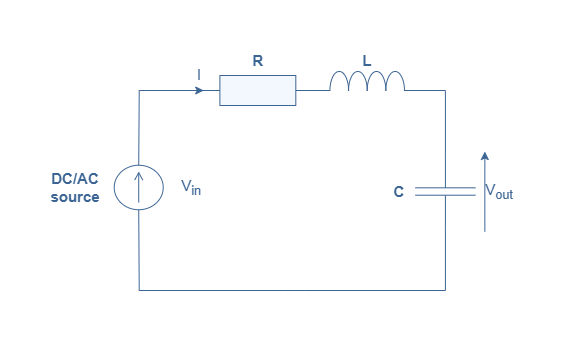
A representation of the RLC circuit is given in Figure 1 below:
fig 1: Illustration of the series RLC circuit
The resistor is a purely resistive component that presents no phase-shift between the voltage and current across it. Its impedance (ZR) remains the same in DC and AC regime and is equal to R (in Ω).
The inductor is a purely reactive component with a phase-shift of +90° or +π/2 rad. Its impedance is given by ZL=jωL with ω being the angular pulsation of the voltage/current in an AC situation and L is the inductance (in H). In the DC regime, an inductor behaves as a short-circuit between two terminals and in the AC regime it becomes an open-circuit as the impedance increases with the frequency.
An inductor is often presented as a component that opposes the variations of current.
The capacitor is also a purely reactive component, but its phase-shift is -90° or -π/2 rad. Its impedance is given by ZC=-j/Cω with C being the capacitance (in F), it behaves therefore as an open-circuit in DC regime and as a short-circuit in AC regime when the frequency increases.
A capacitor is often presented as a component that opposes the variations of voltage.
In Figure 1, these three components are interconnected in series. The circuit is either supplied with a DC or AC source and the output is the voltage across the capacitor. The total impedance of the circuit is the sum of the independent impedances previously stated:
ZRLC=ZR+ZL+ZC=R+j(Lω-(1/Cω))
In the next section, we present the response of this circuit to a voltage step also known as the transient response.
Transient response
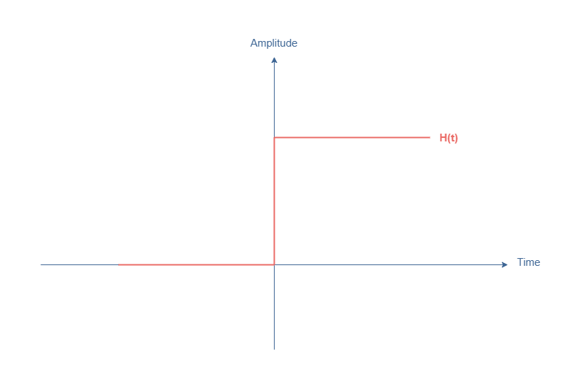
In this section, we will focus on the behavior of the circuit presented in Figure 1 when applying a Heaviside step H(t) to it:
fig 2: Illustration of the Heaviside function
The Heaviside step is characterized by being equal to 0 for t<0 and Vin for t>0. The transition between these two states is similar to an impulsion since the derivative tends to +∞ when t=0.
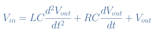
By doing a mesh analysis on the circuit, we can write that Vin=R×I+L×dI/dt+Vout. Moreover, we know that the current can be rewritten I=C×dVout/dt, which leads to the following second-order differential equation:
eq 1: Second-order differential equation of the series RLC circuit
The solution to such an equation is the sum of a permanent response (constant in time) and a transient response Vout,tr (variable in time). The permanent response is easy and obvious to find, the solution Vout=Vin is indeed a permanent solution of Equation 1.
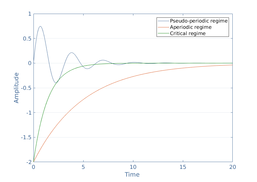
The transient response is complex to determine and involves many steps that will not be detailed in this article. We will admit that its expression can take three different forms and depends on the value of Q=(1/R)√(L/C) called the quality factor of the circuit. Another important parameter is ω0=1/√(LC) which is the fundamental pulsation of the circuit.
When Q>1/2, the regime is said to be pseudo-periodic or to be an underdamped response, the transient response can be written with the form Vout,tr=Ae-αtcos(ωt+Φ). The constants A, α and Φ can be found by considering the initial conditions of the circuit (if the capacitor is charged or not …). The pulsation ω is called the pseudo-pulsation and depends on the fundamental pulsation ω0.
When Q<1/2, the regime is said to be aperiodic or to be an overdamped response, the transient response takes the form Vout,tr=e-αt(A1e-ωt+A2eωt).
Finally, the last case when Q=1/2, which corresponds to the critical regime or critically damped response. In this case, Vout,tr=(A+Bt)e-ω0t.
What is important to keep in mind is that these different solutions dictate how the voltage Vout behaves and tends to its permanent value Vin when a Heaviside step is applied to it:
fig 3: Curves of the different regimes for the transient response
We can comment on this figure by starting to say that each curve tends to 0 when the time increases. It makes sense because we know that Vout=Vin+Vout,tr and Vout(t→+∞)=Vin, therefore, Vout,tr→0.
However, the different possible transient responses do not tend to 0 with the same speed and behavior. The critical regime is the regime that tends the fastest to 0 meanwhile the aperiodic regime is the slowest. The pseudo-periodic regime presents oscillations which amplitude decreases exponentially.
For an unknown RLC circuit, identifying and matching the transient response with the best possible curve can give us the important properties of the circuit such as ω0and Q.
AC response
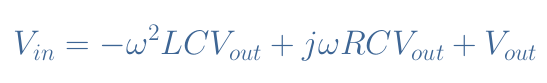
We consider in this section the same circuit presented in Figure 1 now supplied with an AC source. Using the property that in the complex notation, dX/dt=jωX with ω being the angular pulsation of the source, we can rewrite Equation 1 under the following form:
eq 2: Complex second-order differential equation of the series RLC circuit
We can then express the ratio Vout/Vin which is the transfer function T of the series RLC circuit:
eq 3: Transfer function of the series RLC circuit
Knowing that Q=(1/R)√(L/C), ω0=1/√(LC) and considering the parameter x=ω/ω0 called the reduced pulsation, we can rearrange Equation 3 to write the canonical form of the transfer function which simplifies and makes the expression more compact:
eq 4: Canonical form of the transfer function of the RLC circuit
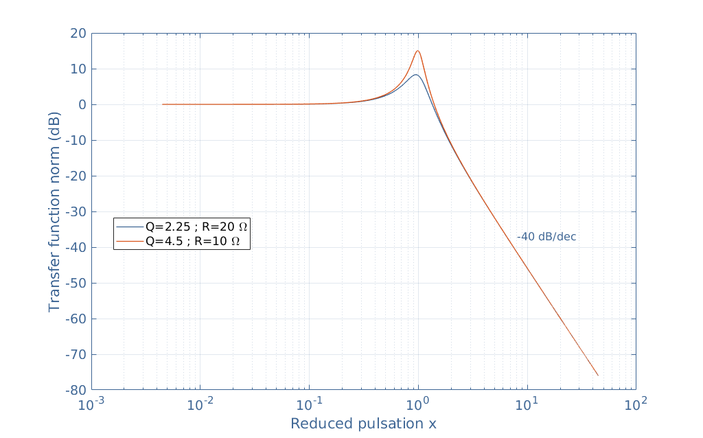
It is interesting to plot the norm of the transfer function in order to obtain the gain of the circuit as a function of the parameter x. The values R=10 Ω and 20 Ω, L=0.2 H, and C=100 μF have been taken for this example:
fig 4: Gain of a series RLC circuit
We can note that the series RLC circuit presented in Figure 1 acts as a second-order low-pass filter in the AC regime since it decreases the output signal for the pulsations higher than ω0, which is commonly called the resonance frequency of the circuit.
Second-order filters have the property to slightly amplify the signal for the frequencies around ω0 and present a decrease of -40 dB/dec after the cutoff frequency, instead of only -20 dB/dec such as for first-order filters.
It is highlighted in Figure 4 that the value of Q (which depends on R) as an effect on the shape of the curve. The peak around the resonance frequency is indeed characterized by its bandwidth Δω=ω0/Q.
In this example, ω0=223 rad/s and Q=4.5 or 2.25, which gives a narrower bandwidth of Δω=50 rad/s for the orange curve and a wider one of 100 rad/s for the blue curve. We can, therefore, note that the quality factor dictates if the resonance is narrow (large Q) or wide (small Q).
Such as mentioned in the previous section, fitting the transfer function of an unknown circuit with the best possible curve enables us to have access to the properties of the circuit and therefore determine the value of its constitutional components.
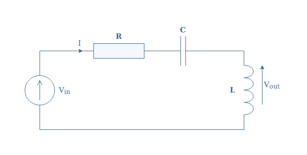
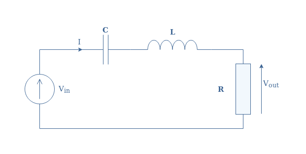
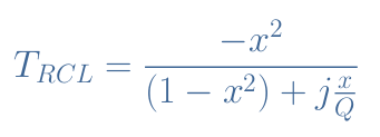
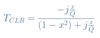
RCL and CLR configurations
Other associations of the elementary component R, L, and C can provide different types of filters. We have seen previously that an RLC configuration is a second-order low-pass filter, but what if we switch some components between them?
Figures 5 and 6 present two new configurations which will be referred to as RCL and CLR circuits:
fig 5: Illustration of the RCL circuitfig 6: Illustration of the CLR circuit
Despite the small changes between these circuits and the original RLC circuit presented in Figure 1, the AC responses are very different.
It can indeed be shown that the transfer functions of these two circuits are given by Equations 4 and 5:
eq 5: RCL circuit transfer functioneq 6: CLR circuit transfer function
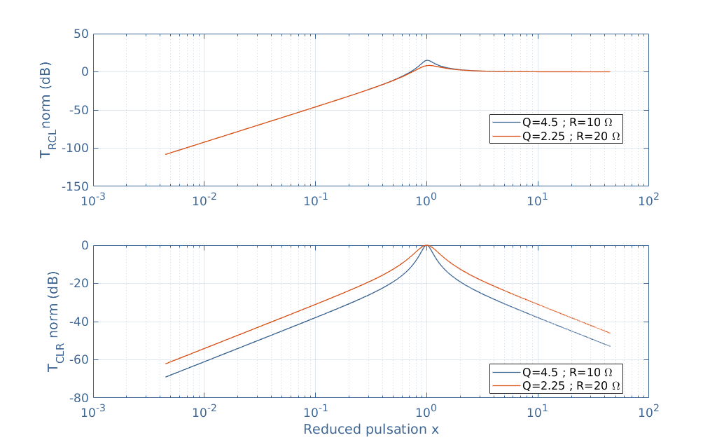
The nature of these new filters is revealed by plotting the norm of their transfer function with the same values: R=10 Ω and 20 Ω, L=0.2 H, and C=100 μF.
fig 7: Gain of series RCL and CLR circuits
The circuit RCL is a second-order high-pass filter since it attenuates the frequencies under ω0. The circuit CLR is a band-pass filter since it only amplifies frequencies in around ω0. Note that the same commentaries as in the previous section about the shape of the curve as a function of Q still apply for both these filters.
Conclusion
The series RLC circuit is simply an association in series of the three elementary components of electronics: resistor, inductor, and capacitor. The impedance of a resistor is a real number and the impedances of the inductor and capacitor are pure imaginary numbers, the total impedance of the circuit is a sum of these three impedances and is, therefore, a complex number.
The transient response of the circuit is first defined and presented in a second section. It consists of investigating the behavior of the circuit when supplied with a Heaviside voltage step. Through studying the possible solutions of the second-order differential equation associated with the circuit, three regimes appear to be possible:
The underdamped response where the signal slowly oscillates towards the permanent value Vin.
The overdamped response where the signal slowly increases towards the permanent value.
The critically damped response is the scenario where the signal increases the fastest towards the permanent value.
In a third section, the AC response of the circuit is presented. When supplied with an AC signal, the differential equation can be written in its complex form in order to find the transfer function of the circuit. Plotting the norm of this function reveals that the series RLC circuit behaves as a second-order low-pass filter.
In the last section, alternative configurations called RCL and CLR are investigated. This section shows that a second-order high-pass filter or a band-pass filter can be made from the same circuit by simply switching the components.
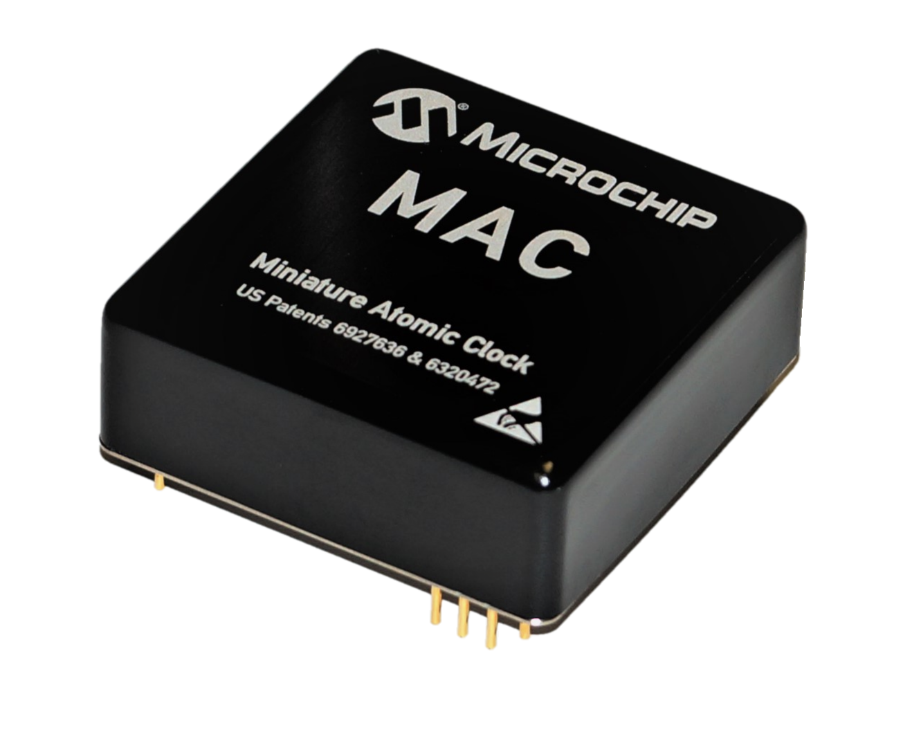
Miniature Atomic Clock (MAC – SA5X) Rubidium Oscillator, re-designed for improved stability and new features. The MAC-SA5X is designed for applications that require long-term atomic oscillator stability, but are constrained by size and low power requirements.
Versatile
Microchip’s next-generation MAC-SA5X miniaturized rubidium atomic clock produces a stable time and frequency reference that maintains a high degree of synchronization to a reference clock, such as a GNSS-derived signal, despite static g-forces or other factors. Its combination of low monthly drift rate, short-term stability and stability during temperature changes allow the device to maintain precise frequency and timing requirements during extended periods of holdover during GNSS outages or for applications where large rack-mount clocks are not possible.
Compact Design
Sharing an identical form factor with the Legacy MAC, measuring only 2 inch by 2 inch and standing less than an inch – it is five times smaller than traditional lamp-based rubidium oscillators. Its pins allow it to be mounted to PCBA’s.
Improved Operation
It has been designed for fast warm-up times in a variety of thermal environments, wider operational temperature range and improved stability performance.
Low Temperature Sensitivity
With a max frequency deviation of <5E-11 during large temperature changes, along with improved long-term drift rates, the MAC-SA5X is capable of sub-microsecond holdover for many days in variable environments.
Additional Features
1PPS Disciplining allows fast calibration to external references, such as GNSS-derived 1PPS signals. New software interface adds user-versatility, control and monitoring of the device via rs232 or USB communications pins.
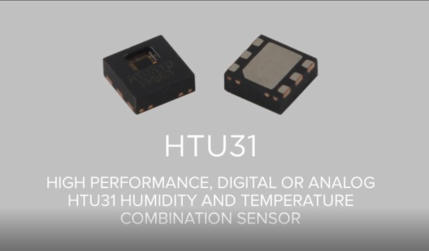
TE Connectivity released the HTU31 humidity and temperature sensor, presented as one of the smallest and most accurate humidity sensors currently available. The sensor provides precision measurement, fast response time, low hysteresis, and sustained performance, even in harsh environments.
The HTU31 keeps a strict linear response curve through its humidity (0-100%) and temperature (-40° to 125°C) ranges, respectively, and its humidity die structure enables a response time of t63% in 5 sec. Even after condensation the response time is t63% in 10 sec.
Key features of the HTU31 humidity and temperature sensor include:
Precision engineering: Designed with precision engineering, HTU31’s linear response enables optimal system performance. It keeps a strict linear response curve through humidity (0-100%) and temperature (-40° to 125°C), respectively.
Fast response time: HTU31’s humidity die structure enables fast response time (t63% in 5 sec). Even after condensation the response time is t63% in 10 sec, enabling sustained system performance.
High performance: HTU31 provides a specific die and IP67 rated sealing with filter options that enable sustained performance, low hysteresis and precise environment measurement even when exposed to high temperature, high humidity or condensation events.
Digital and analog versions: The HTU31 comes in a digital and analog version. The digital version offers two I2C addresses, which facilitates monitoring humidity and temperature in two locations using a single I2C bus line.
The IP67-rated device offers filter options for sustained performance, low hysteresis, and precise environment measurement under high temperature, high humidity, or condensation events. The HTU31 comes in a digital model with two I2C addresses, and an analog version.
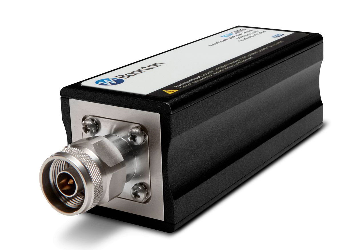
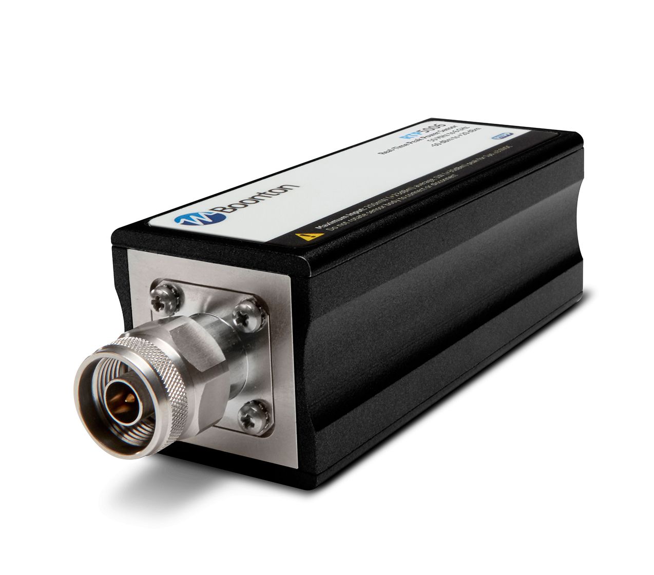
RTP5000 Real-Time Peak Power Sensors provide high video bandwidth, fast rise-times, and unique Real-Time Power ProcessingTM to deliver 100,000 RF measurements per second, with no gaps in signal acquisition, and zero measurement latency.
Saelig Company, Inc. has introduced the Boonton RTP5000 Series Real-Time Peak Power Sensors, offering industry-leading performance with wide video bandwidth, fast rise times, fine time resolution, narrow minimum pulse widths, high pulse repetition rates, and superior measurement reading rates. These USB-connected RF power sensors incorporate Boonton’s unique Real-Time Power Processing™ technology, which delivers measurements with no gaps in signal acquisition and zero measurement latency. RTP5000 Peak Power Sensors provide fast, accurate, and reliable RF power sensing, with automatic pulse measurements.
The RTP5000 series features 100ps time base resolution with an acquisition rate up to 100MSa/s, providing 50 points per division with a time base range as low as 5ns/div, gathering useful waveform information often missed by other power analyzers. Pulse widths as narrow as 10ns can be captured and characterized with outstanding trigger stability (< 100psRMS jitter).
Real-Time Power ProcessingTM (RTPP) technology is a unique parallel processing methodology that rapidly performs the multi-step process of RF power measurements. Competing conventional power meters and USB sensors perform measurement steps serially, resulting in long re-arm times and missed data. RTP5000 sensors can capture, display, and measure every pulse, glitch and detail with no gaps in data and zero latency. A Measurement Buffer Mode works in conjunction with Real Time Processing to allow users to collect and analyze measurements from a virtually unlimited number of consecutive pulses or events. A wide variety of parameters can be calculated and plotted (e.g. duty cycle, pulse repetition rate, pulse width variation, pulse jitter, etc.) Anomalies, such as dropouts, can also be identified.
To simplify test procedures, the RTP5000 series can measure, calculate, and display sixteen common power and timing parameters, including rise time, fall time, pulse average, overshoot, and droop. The Boonton Power Analyzer software package, provided free, allows users to use the complementary cumulative distribution function (CCDF) to assess the probability of various crest factor values to gain further insight into DUT performance. The CCDF and other statistical values are determined from a very large population of power samples captured at a 100MSa/s acquisition rate on all channels simultaneously.
6GHz/18GHz/40GHz RF Power Sensors
Up to 195MHz video bandwidth with 3ns rise time
Real-Time Power ProcessingTM technology
Zero measurement dead time
100,000 measurements/sec
Crest factor, CCDF, statistical power measurements
Five models in the RTP500 series cover 50MHz to 40GHz measurements: RTP5006 (50MHz – 6GHz), RTP5318 (50MHz – 18GHz), RP5340 and RP5540 (50MHz – 40GHz). With superior performance and a small form factor, the Boonton RTP5000 series is ideal for design and verification, manufacturing, field installation and maintenance. The sensors can effectively measure pulsed, bursted, and/or modulated signals used in commercial and military radar, electronic warfare (EW), wireless communications(e.g., LTE, LTE-A, and 5G), and consumer electronics (WLAN), as well as in education and research applications.
Made by Boonton Electronics, a recognized leader in high-performance RF test instrumentation and sensors, the RTP5000 Series Real-Time Peak Power Sensors are available now from Saelig Company, Inc. their USA technical distributor.
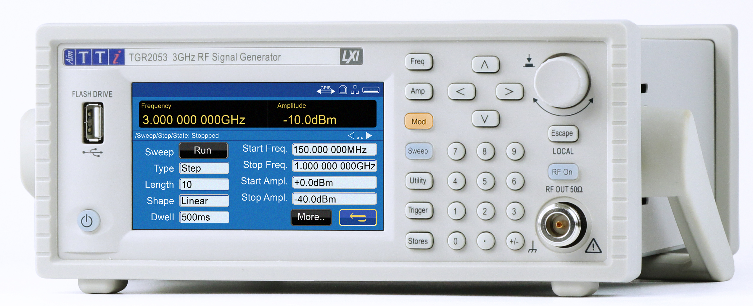
The TGR2051/2053 RF signal sources provide exceptional performance with touch-screen operation for improved functionality to support research and development, test and service applications
Saelig Company, Inc. announces the availability of the AIM-TTi TGR2051 and TGR2053 RF Signal Generators, a major revision of their successful TGR 2000 series, which both offer exceptional performance, very low phase noise, and flexible functionality, offering output signals from 150kHz to 1.5 and 3GHz respectively. These versatile RF generators provide excellent frequency accuracy and stability, large signal amplitude range, low phase noise and extensive analog and digital modulation capabilities. Output power levels from -127dBm to +13dBm are available with 50VDC reverse voltage protection.
Both models feature a simple, user friendly, touch-operated GUI, with the 4.3” color LCD clearly showing all relevant information and settings. Parameters can be adjusted from the menu on the LCD touch-screen or by using the front-panel keys and rotary wheel. A front-mounted USB flash drive allows pre-defined complex setups, sweep lists, and modulation patterns to be loaded into the instrument quickly and efficiently. 4GB of non-volatile internal memory is provided for storing multiple setups, sweep lists, arbitrary modulation patterns and more. Up to 1000 complete setups can be stored internally.
The instrument’s built-in DDS generator provides sine, square, +ramp, -ramp and triangle waves, and these can be applied in AM, FM or PM from the internal modulation source at frequencies ranging from 1mHz to 1MHz. External analog modulation signals can be applied via the rear panel. An extensive number of digital modulations are also available: FSK, GFSK, MSK, GMSK, HMSK, 3FSK, 4FSK, PSK, ASK and OOK. Built in NRZ patterns include square wave, 7, 9, 11 & 15-bit PRBS. Digital modulation capabilities also include advanced filtering: Gaussian, Raised Cosine, Root Raised Cosine and Half Sine, as well as Grey Code and Binary Encoding. External digital modulation signals can be applied to the carrier waveform via the rear panel. A user-defined pattern generator is also included for modulating the carrier signal. Digital modulation and modulation patterns can be continuous or triggered externally, internally, manually, or remotely.
The sweep function can vary frequency and/or amplitude to test a wide range of input conditions. Linear or logarithmic sweeps can operate upwards or downwards. Alternatively, List Mode can be used to analyze a response at set frequencies and amplitude, dwelling on set values for specified periods. This technique is useful for tests at specific suspected problematic frequencies. Complex sweep triggering can control complete sweeps and/or each point within a sweep.
Both signal generators offer advanced remote-control connectivity for use in sophisticated automated systems. These RF sources can be rack-mounted with an available 2U 19” rack kit. They can be integrated into existing or new test setups with the help of an extensive command library for SCPI systems and Windows drivers for LabView, LabWindows, and Keysight VEE applications. Backward compatibility with Aim-TTI’s previous RF instruments enables their use in legacy systems too.
The TGR2051/2053 generators provide exceptional performance with high signal purity, high frequency accuracy and stability, a large signal amplitude range, low phase noise and fast amplitude/frequency sweeps. Extensive and flexible analog and digital modulation capabilities make these signal generators ideal for research and development, test and service work. With a small footprint and lightweight design, the TGR2051/2053 generators are high quality, reliability, and great value instruments for electronic design and test engineers. Made by Aim-TTi, a leading European test equipment manufacturer, the TGR2000 series of RF signal generators is available now from Saelig Company, Inc., Fairport, NY their technical distributor.
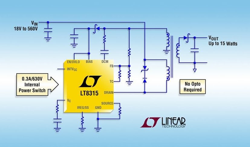
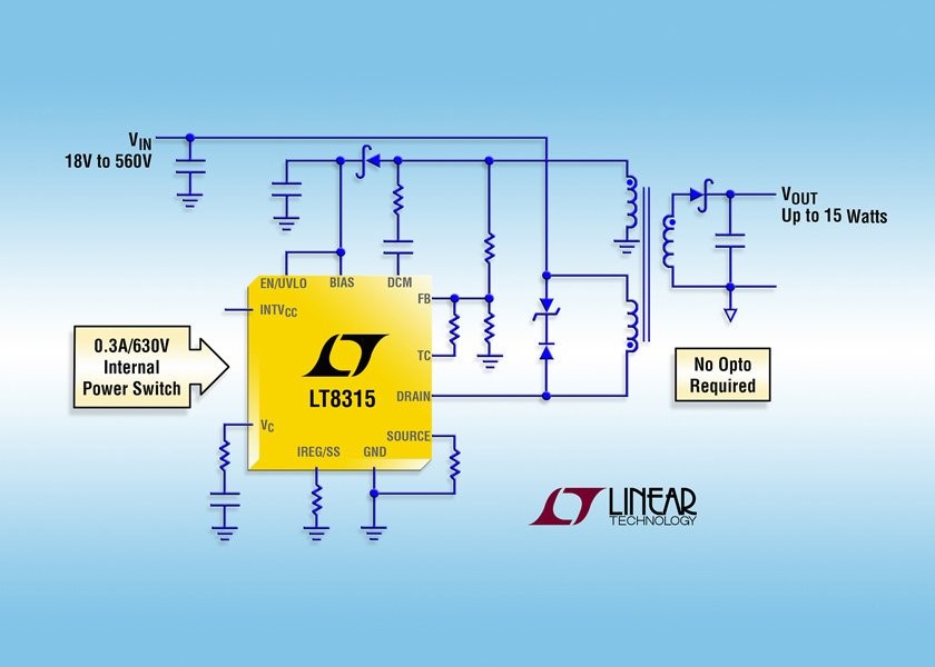
Linear Technology’s 560 VIN micropower no-opto isolated flyback converter with 630 V / 300 mA switch
Linear Tech’s LT8315 high voltage flyback converter with integrated 630 V / 300 mA switch needs no opto-isolator for regulation. It samples the output voltage from the isolated flyback waveform appearing across a third winding on the transformer. Its quasi-resonant boundary mode operation improves load regulation, reduces transformer size, and maintains high efficiency. At start-up, the LT8315 charges its INTVCC capacitor via a current source attached to the DRAIN pin. The current source turns off and the device draws its power from a third winding on the transformer during normal operation. It operates from a wide range of input supply voltages and can deliver up to 15 W of power. The LT8315 is available in a thermally enhanced 20-pin TSSOP package with four pins removed for high-voltage spacing.
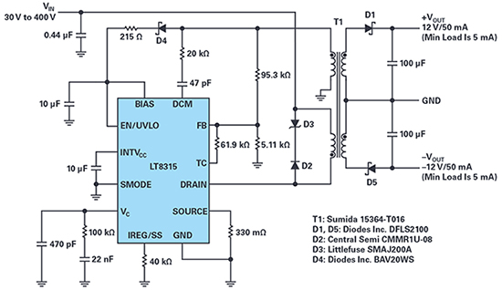
A complete ±12V/50mA isolated flyback converter for a wide input range, 30V to 400V
The STM32L5 microcontroller series is the solution and provides a new optimal balance between performance, power, and security
Security has emerged as one of the 3 key areas that developers of embedded and IoT applications are thriving to improve. The STM32L5 microcontroller series is the solution and provides a new optimal balance between performance, power, and security. The STM32L5 MCU series harnesses the security features of the Arm Cortex-M33 processor and its TrustZone for Armv8-M combined with ST security implementation. ST-proprietary ultra-low-power technologies create a class-leading MCU for energy-conscious applications such as the Internet of things (IoT), medical, industrial and consumer.
Key features
More Security with TrustZone Security and ST Security Implementation
Lower Power Consumption
Integration, Size, Performance: More performance, Large Memory Size and Wide Portfolio
A Full Set of Security Options
Additional features
A full set of security options:
Flexible hardware and software secure isolations with TrustZone
Enhanced security services:
dedicated secure user memory space for Secure Boot, symmetric and asymmetric crypto accelerations, memory and IP protection
independent readout protection between secure/non-secure domains, active I/O tamper detection
certified crypto lib, embedded Secure Firmware Install loader and ecosystem.
Low power consumption:
EEMBC ULPBench®: 402 ULPMark-CP score
Embedded SMPS step down converter (optional)
Best power consumption numbers with full flexibility:
33 nA in shutdown mode
3.6 µA in stop mode with full SRAM and peripheral states retention with 5µs wake-up time
Down to 60 µA/MHz in active mode
Integration, size, and performance:
Better application responsiveness:
New Arm® Cortex®-M33 at 110 MHz performance: +20% versus Cortex®-M4
New ST ART Accelerator: working both on internal and external Flash (8 Kbytes of instruction cache)
Capable of achieving 165 DMIPS and 442 CoreMark scores
High integration and innovation: large memory, USB Type-C with power delivery controller, CAN FD
Large portfolio: 7 package types (LQFP48, QFN48, LQFP64, WLCSP81, LQFP100, UFBGA132 and LQFP144)
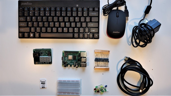
The “Sania Box Embedded Computer Kit” was developed by Sania Jain, a 13-year-old writer who has a passion for coding. The project was launched with the help of a Silicon Valley-based start-up called MoonShot Junior Inc. The goal of the project is to help children learn or improve coding and STEAM (Science, Technology, Engineering, Art, and Mathematics) skills without adult supervision.
The Sania box comes with an embedded add-on board that comes with amazing features like pushbuttons, sensors, and even a relay circuit. The board fits on a Raspberry Pi 3 or Pi 4 board 40 Pin header. It also comes with an SD card that has pre-installed code for kids to practice with. Other attachments that come with the add-on board are:
Two LED Lights
3 -digit – 7 Segment Clock Display
Light Sensor
Gas Sensor
Thermal Sensor
Touch Sensor
Relay and Audio Buzzer
Push Button4
Sania Box – Embedded Computer Kit
Kids can bring their program to life by putting the various components of the board. This is a very powerful educational tool, especially for computer science programming and engineering.
Python has been chosen as the preferred programming language for the board. This is an excellent decision as python is easy to understand and expressive. Younger programmers with little or no experience will find it easy to learn. The kit is based on a Raspberry Pi 4, so it will work with every other language supported by Raspberry Pi 4.
The box is a DIY project which targets children who are 8 years old or older. They can create projects based on their codes. The kit comes with a keyboard, mouse, and custom case. The breadboard, LEDs, and resistors, which are included, make the Sania box a great resource. There is no need to search for other components before creating a complete project.
Sania Box – Embedded Computer Kit
Although there is no display provided, the Sania box has an HDMI cable included which offers the option of connecting to a television in a classroom setting or any other display available.
Pricing and Further Information
Coding is a 21st Century skill, which is essential. Most schools do not have a chance to offer computer programming to students, and the Sania box will be a fantastic way to tackle this problem. There is currently a $129 pledge offer available on Kickstarter for the first 200 boxes. After that, the Sania box will be sold for $149, and other donations are welcome.