There are thousands of different electronic component distributors and suppliers around the world, who sell similar parts with a range of different prices. However, In the course of my internet search, i stumbled upon WIN SOURCE, a Hong Kong-based electronic component distributor of commonly-used components and obsolete parts since 1999. They boast of over hundreds of thousands of different electronic parts, with a pocket friendly price, especially if you are purchasing in bulk or individually.
They distribute and manufacture over 100 popular brands, over 500,000 SKUs stock. 365-day with 24 hours shipment is a bright spot. They also passed several authoritative quality certifications, including AS9120, ISO9001, ISO14001 at the same time.
Win-Source Electronics various Certifications
It is not only popular for their excellent services, certifications and website, they are also popular for the quality of their components as. Customer reviews shows that they have been satisfied with Win Source for its quality components and fast delivery. Any part you purchase has a one year warranty in case of anything is defective or wrong with them, coupled with their 24 hours delivery service, that making it one of the reasons why I would also recommend the company to all electronic enthusiast.
In order to purchase any component through their website, you have to create an account. It is a very simple process, they just need a few details. Creating an account enables you to receive personalized newsletters, and update you on everything which is going on.
WIN SOURCE’s website is very detailed and easy to navigate, with the catalog displaying the whole shop’s inventory, part-by-part, and also displaying the individual SKU, Ladder price and detailed description, etc.
It is worth mentioning that when I browsed the specification list, I found several special parameters, Fake Threat In the Open Market and Supply and Demand Status. This will be a valuable parameter for engineers in purchasing and purchasing. You can also check the ECAD Module and alternative parts recommendations.
They went a step further by operating a customer service email and a live chat service on their website, which is very convenient service for buyers. One aspect that is very user-friendly is that WIN SOURCE provides users with free electronic component campaign, which is really exciting for engineers who have difficulty selecting models or companies that produce sample tests.
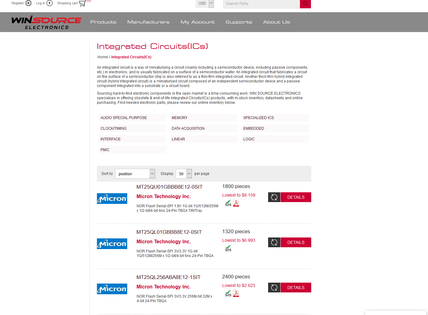
They have various manufacturers under one site, so if for example I’m looking for integrated circuit products, when i search for it, it brings up various companies selling integrated circuits product page. This makes it easy for me to pick from a variety of products.
Another noteworthy service rendered by the company is their Return Policy which is reasonable, and also an Environmental, Anti-Counterfeit and Privacy Policy, to reassure you that they a trusted website to use. WIN SOURCE makes sure they maintain a high standard between them and their customers. Their payment methods include: VISA, Mastercard, American Express and PayPal, which are all secure and simple mediums for payment.
Search results on Integrated Circuits on Win-Source Electronics site
One interesting part of Win Source’s website, is the news section of it, there you can find the latest updates and news about what’s going on in the world of electronic components. News about the latest brands, updates about components and much more can be found on the news page on the website. They provide updates on the page regularly, so you can endeavor to visit the site every week.
In summary, I highly recommend Win Source Electronics products and services to all who are interested in purchasing products from them. They are a genuine and experienced company, they are capable of catering to the need of everyone, either those who are newbies in electronics, or people who are experienced in the electronics industry. You have a massive selection to choose from, this makes Win Source your go to for electronics. You can send an email to their support team, they are very friendly, and ready to answer all your questions, and provide you with the necessary information which you need. Visit Win Source Electronics’ website for more details and user experience.
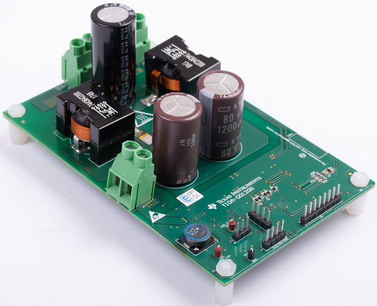
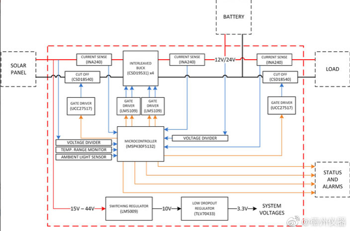
This reference design is a Maximum Power Point Tracking (MPPT) solar charge controller for 12-V and 24-V solar panels. This compact reference design targets small and medium power solar charger solutions and is capable of operating with 15- to 60-V solar panel modules, 12- or 24-V batteries and providing upwards of 20 A output current. The design uses a two-phase interleaved buck converter to step down the panel voltage to the battery voltage. The buck converter and its connected gate drivers are controlled by a microcontroller unit (MCU), which calculates the maximum power point using the perturb and observe method. The solar MPPT charge controller is created with real-world considerations, including reverse battery protection, software programmable alarms and indications, and surge and ESD protection.
Features
96% efficiency in 12-V systems and 97% efficiency in 24-V systems
Wide input voltage range: 15 V to 60 V
High rated output current: 20A
Battery reverse polarity, over-charge and over-discharge protections
System over-temperature and ambient light detection capabilities
Small board form factor: 130 mm x 82 mm x 38 mm
TIDA-010042 MPPT charge controller reference design for 12- and 24-V solar panels block diagram image
LaserPecker recently announced a Pro version of their LaserPecker portable, affordable, compact laser engraver. Launched earlier this week on Kickstarter, the Laspecker Pro surpassed its modest funding goal of $10,000 in just 14 minutes and is currently approaching $200,000 with over three weeks left to go in the campaign. LaserPecker states their engraver can burn images, words, and patterns on nearly every material — food, metal, plastic, leather, and more.
According to the company,
“LaserPecker Pro is upgraded with an auto-adjusting support stand that sets up and focuses in seconds. All you have to do is put the engraving target on the spot. The built-in sensors of the stand will measure the distance between the laser generator and the target and automatically adjust the height to make sure the focal point is the correct distance from the surface of the object.”
LaserPecker upgraded the laser on the Pro version from a 450nm blue laser with 0.3mm light spot to a 450nm blue-violet laser with 0.15mm beam, which the company claims has over a 10,000-hour working lifespan. The Pro is a plug-and-play engraver ready to go outside the box and can use multiple power sources, including wall outlets, battery packs, and via USB Type-C cable.
Intro Video
As mentioned earlier, the LaserPecker Pro laser engraver is available now on Kickstarter with pledges starting at $269, which includes the engraver, safety goggles, materials package, magnetic protective shield, USB cable, and tripod stand. At the $369 level, you get the same goodies box, only it comes with the auto-focus support stand as well.
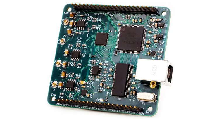
simpleFE is a low cost, fully open-source, mixed-signal front-end. Designed primarily to carry out analog-to-digital and digital-to-analog conversion, simpleFE includes plenty of IO and allows you to create your own signal processing system more quickly, more easily, and more cost-effectively.
Features & Specifications
ADC: 8-bit, two channels, up to 7.5 Msps (I and Q)
DAC: 10-bit, two channels up to 7.5 Msps (I or Q) or 5 Msps (I and Q)
USB: High speed interface (USB 2.0)
GPIO: 16 pins
DAC Output: 10-bit, four pins
SPI: One interface
I²C: One interface
Antenna Connectors:
Two U.fl analog output (50 Ohm output impedance)
Two U.fl analog input (high impedance)
Components
USB: EZ-USB FX2LP (CY7c68013A)
FPGA: ICE40HX1K
Front-end: MAX5863
Software: GNURadio, gr-simplefe, libsimplefe C library
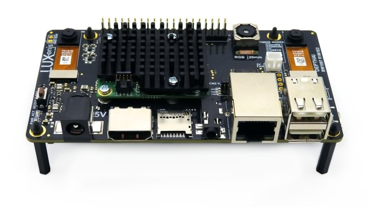
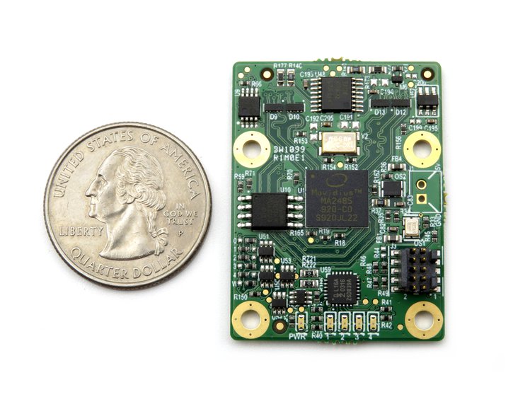
DepthAI is a platform built around the Myriad X to combine depth perception, object detection (neural inference), and object tracking that gives you this power in a simple, easy-to-use Python API. It’s a one-stop shop for folks who want to combine and harness the power of AI, depth, and tracking. It does this by using the Myriad X in the way it was intended to be used – directly attached to cameras over MIPI – thereby unlocking power and capabilities that are otherwise inaccessible.
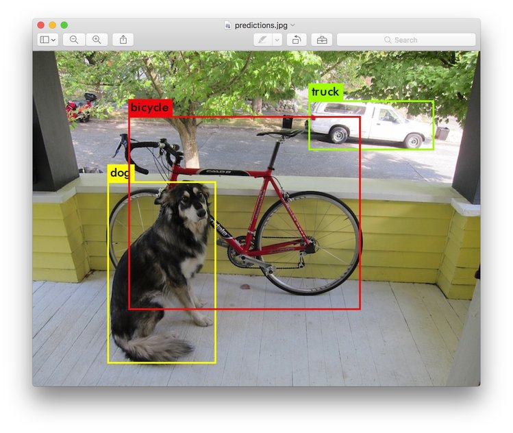
Real-time Object Localization
Object Detection is a marvel of Artificial Intelligence/Machine Learning. It allows a machine to know what an object is and where it is represented in an image (in ‘pixel space’).
Back in 2016, such a system was not very accurate and could only run at (rougly) one frame every six seconds. Fast forward to 2019, and you can run at real-time on an embedded platform – which is tremendous progress! But, what good does knowing where an object is in an image in pixels do for something trying to interact with the physical world?
That’s where object localization comes in. Object localization is the capability to know what an object is and where it is in the physical world. So, its x, y, z (cartesian) coordinates in meters.
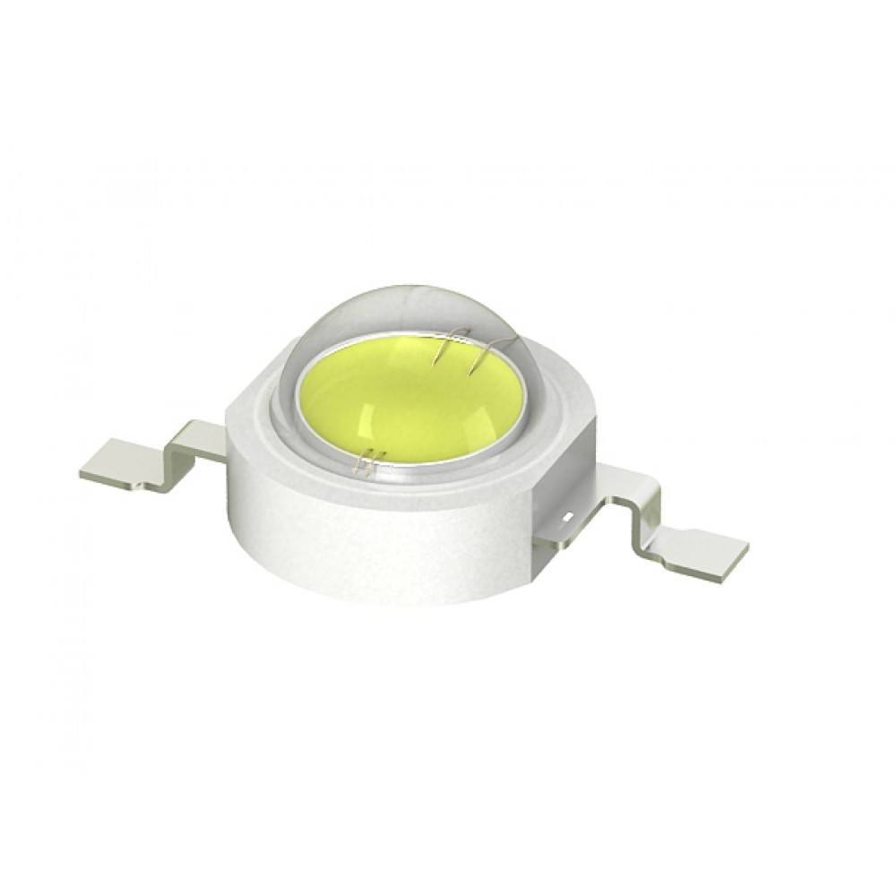
This flasher/beacon circuit can be employed as a distress signal on highways, a direction pointer for parking lots, hospitals, and hotels, etc. The circuit uses a power LED, and provides more light than a typical incandescent lamp flasher. Use of a 6 V or 12 V SLA lantern battery makes the circuit portable.
The heart of the circuit is an MC34063 monolithic switching regulator subsystem, originally intended for use in DC-DC converters (Figure 1). This device contains a voltage reference, comparator, controlled duty cycle oscillator with an active peak current limit circuit, driver, and a high current output switch, all in an 8-pin DIP.
Figure 1. Functional Diagram of the MC34063.
The circuit briefly flashes a 1 W power LED from a 6 V to 12 V DC supply – at about 5% duty-cycle (Figure 2). Current limiting to the LED is accomplished by monitoring the voltage drop across R1, a 1 W sense resistor placed between VCC and the output switch, pin 1.
Figure 2. The Schematic Diagram of a Flashing Beacon.
The maximum current capability of a 1 W white LED is about 350 mA. At the beginning of a cycle, C1 starts to charge, and LED current rises rapidly, along with the drop across R1 which is monitored by the Ipk sense pin, IC1-7.
When this voltage becomes greater than 330 mV with respect to pin 6 (i.e., 330 mA), the current limit block in the IC provides additional current to charge the timing capacitor C1. This causes it to rapidly reach the upper oscillator threshold, at which point the output switch turns off and C1 discharges. Flashing rate can be altered by changing the value of C1. 100 µF gives approximately 4 Hz.
Since the LED flashes on very briefly, thermal issues are minimal and a star MCPCB is sufficient to cool the LED.
With digital semiconductor technology driving system power supplies to lower voltages for higher performance and lower system power, sensitive analog sensor circuits face a growing problem. Much of the inherent noise created in the early stages of an analog sensor signal path is independent of the amplifier bias voltage, so using a higher bias voltage yields better accuracy and performance than a lower bias. With supply voltages dropping, then, designers must tolerate the loss of accuracy (SNR) due to the lower available voltage or derive a higher voltage bias from the available system supply.
In addition to the voltage, designers need to consider the ground. In many cases the sensor circuit must have bias voltages both above and below signal ground. That signal ground can be either a true system ground or a virtual ground created at the midpoint of a single-rail power supply. Using a true system ground requires “split-rail” biasing (±V), but yields improved performance as a result of reduced leakage currents and reduced variations in a virtual ground, both of which affect measurement accuracy.
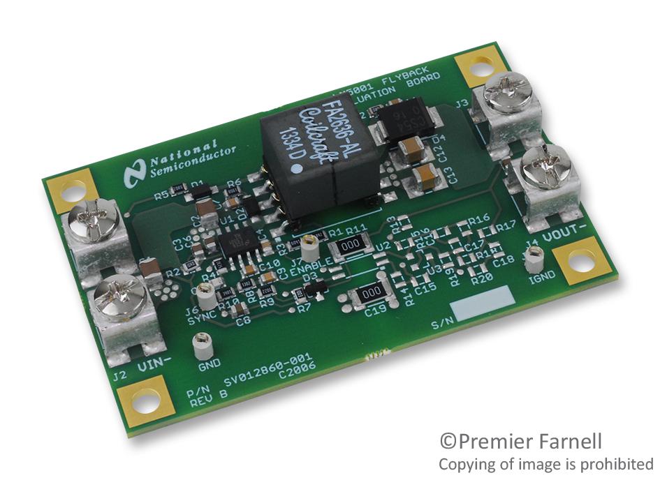
Figure 1. A switch-mode regulator IC and transformer can create ±12-V bias voltages from a system’s 5-V rail to help improve the performance and signal-to-noise ratio of analog sensor front ends.
To obtain the best performance from the analog front end, then, designers need a method of creating a higher voltage split-rail bias from a lower-voltage single-rail supply. One way to create this split-rail voltage is to use a switch-mode regulator IC in concert with a small transformer. This forms a flyback design that uses less than one square inch of board space.
The circuit of Figure 1 boosts a nominal 5-V single-rail supply (4.5 to 5.5 V) to a low-noise, ±12-V bias and can be adapted to develop other voltages such as ±15 V. The design uses a Texas Instruments LM5001 (U1) switch-mode regulator that integrates a pulse-width modulation (PWM) generator, a switching transistor, a voltage reference, and an error amplifier that controls the PWM duty cycle based on a comparison between the reference and the feedback signal on pin 6.
The regulator switches current through the primary of center-tapped transformer T1, and the PWM duty cycle determines the output voltage at the secondary. Diode D3 and its attached components serve as a snubber to minimize transient noise and ringing on the transformer input when the regulator’s internal switch opens. Diodes D2 and D4 serve as half-wave rectifiers for the transformer’s output.
Figure 2. C biasing dominates losses in the split-rail bias circuit at lower currents, but conversion efficiencies greater than 80% are attainable.
Resistor R10 sets the PWM’s nominal switching frequency to 600 kHz, which represents a compromise between conversion efficiency and noise (both switching noise and ripple) on the bias voltage outputs and transformer size. With this frequency, conversion efficiency (Fig. 2) can be greater than 80% depending on load. Both noise and conversion efficiency decrease with increasing switching frequency, so designers can choose to increase efficiency at the expense of noise by adjusting the value of R10. Decreasing the switching frequency often results in the need to increase the size of the transformer, adding to this tradeoff decision.
Capacitors C3, C4, C8, and C9 serve as the principal output filters, but designers can further reduce switching noise by incorporating the optional low-pass post filters L1/C14 and L2/C15 shown on the positive and negative outputs. The filters have a cutoff frequency of about 90 kHz, resulting in less than 10-mV peak-to-peak transient noise and under 2-mV switching ripple measured from dc to 600 MHz. Designers can reduce this noise even further by changing C4 and C9 to 47 µF. Symmetrical layout of the design’s differential power section can help reduce differential noise.
This type of flyback design, which uses only one regulator monitoring the positive output, provides common-mode rejection of some noise components and only uses a single IC. Cross regulation is typically not as tight with one regulator as would be possible when using a separate regulator for the negative output. But since most sensor signal path circuits draw symmetrical current on each rail, cross regulation usually isn’t an issue.
In any case, measurements show good cross regulation with this circuit. Either output maintains regulation to less than 3% when delivering 35 mA while the other output load varies between 10 mA and 50 mA. The design’s measured output tolerance is within 5 mV across both outputs when delivering from 5 to 40 mA from both outputs differentially.
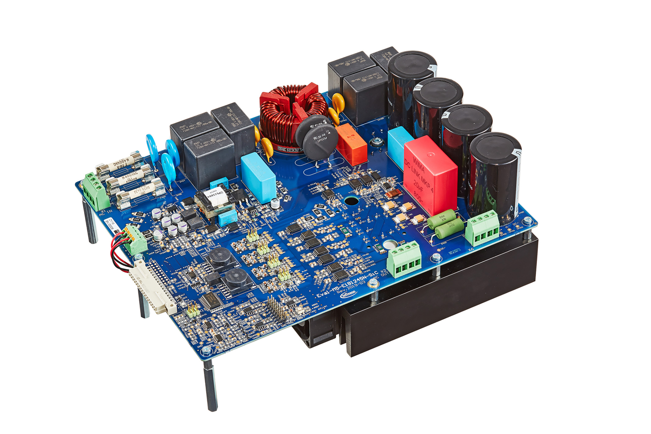
Silicon carbide (SiC) is en route to mainstream for applications like photovoltaic and uninterruptable power supplies. Infineon Technologies AG is now targeting the next group of applications for this wide bandgap technology: The evaluation board EVAL-M5-E1B1245N-SiC will help to pave the way for SiC in motor drives and help strengthening Infineon’s market position as #1 for industrial SiC. It was developed to support customers during their first steps in designing industrial drives applications with a maximum of 7.5 kW motor output.
The evaluation board comprises an EasyPACK™ 1B with CoolSiC™ MOSFET (FS45MR12W1M1_B11), a 3-phase AC connector, EMI filter, rectifier and a 3-phase output for connecting the motor. Based on the Modular Application Design Kit (MADK) the board is equipped with the Infineon standard M5 32-pin interface which allows the connection to a control unit such as the XMC DriveCard 4400 or 1300. Its input voltage covers the range of 340 to 480 V AC.
The new member of the MADK family is optimized for general purpose drives as well as for servo drives with very high frequency. It features the EasyPACK 1B in Sixpack configuration with a 1200 V CoolSiC MOSFET and a typical on-state resistance of 45 mΩ. The power stage contains sensing circuits for current and voltage; it is equipped with all assembly elements for sensorless field oriented control (FOC). The EVAL-M5-E1B1245N-SiC has a low inductive design, integrated NTC temperature sensors and a lead-free terminal plating, which makes it RoHS compliant.
Cypress Semiconductor’s F-RAM is ideal for portable medical, wearable, IoT sensor, industrial, and automotive applications
Cypress Semiconductor’s Excelon is next-generation Ferroelectric RAM (F-RAM) which delivers the industry’s lowest-power mission-critical nonvolatile memory by combining ultra-low-power operation with high-speed interfaces, instant nonvolatility, and unlimited read/write cycle endurance. This makes Excelon the ideal data-logging memory for portable medical, wearable, IoT sensor, industrial, and automotive applications.
Features
Up to 150x reduction in typical standby current (1 µA) and hibernate current (0.1 µA) compared to current F-RAMs
Greater than 10x increase in performance with the addition of a 108 MHz Quad SPI (QSPI) compared to competing SPI F-RAMs
Offers NoDelay™ writes to capture data instantly with no soak time requirement and without any additional components for power back-up
2 Mb, 4 Mb, and 8 Mb density options
Operating voltage range: 1.71 V to 1.89 V and 1.80 V to 3.60 V
Commercial (0°C to +70°C), industrial (-40°C to +85°C), Auto-A (-40°C to +85°C), and Auto-E (-40°C to +125°C) temperature grades
Excelon-LP and Excelon-Ultra individual features
Multiple power-saving modes, including hibernate, deep power-down, and standby
Consume 200x less energy than EEPROM and 3,000x less energy than NOR Flash products
Read/write endurance of 1,000 trillion write cycles to log data every millisecond for more than 3,000 years
Introduce 8 Mb density F-RAM to meet the growing data-logging requirement in modern applications
Available in small footprint: 10 mm², 8-pin GQFN package
Excelon-Auto individual features
Captures data instantly with no soak time requirement and also no additional back-up components
Supports endurance cycling of 1,000 trillion write cycles to log data every µs for 20 years
Provides AEC-Q100-qualified and functional safety-compliant memory components
Example applications
Excelon-LP for portable medical, wearable, and IoT device applications: provides extended battery life, high reliability, and small form factor
Excelon-Ultra for industrial automation systems: ideal memory for highly demanding data-logging needs of PLC
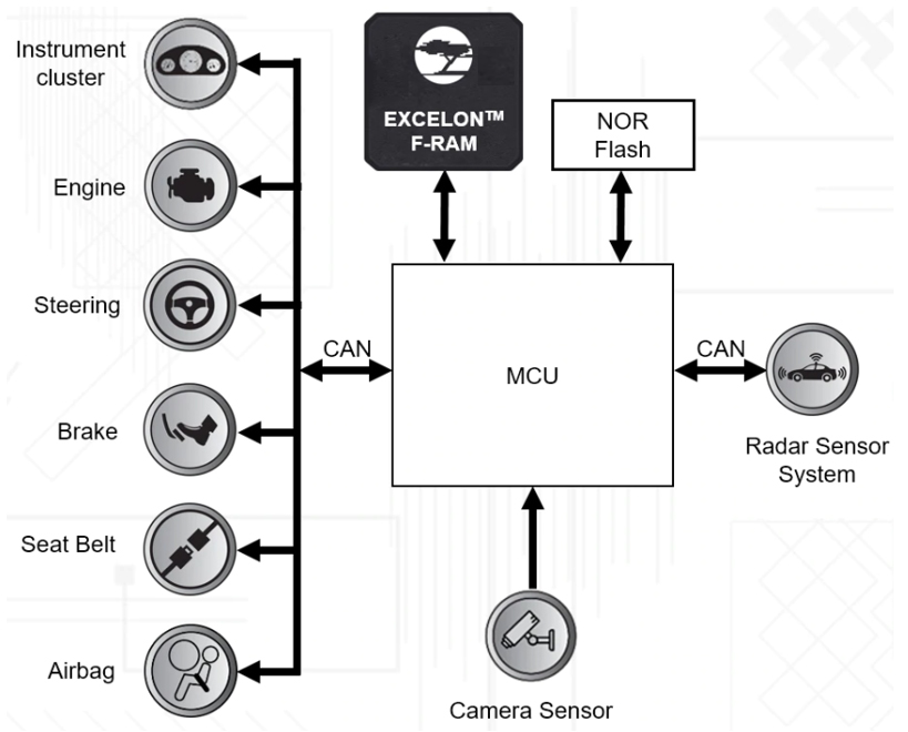
Excelon-Auto for automated driver-assist systems: enables instant and reliable data capture in ADAS vision systems
Complex numbers are an important mathematical tool that is widely used in many physics domains, including electronics. The concept might seem odd, but their manipulation is simple and their efficiency notable.
In the first section, general concepts about the complex numbers are presented in order to get familiar with their representation. A second section will follow by enumerating some of the most important definitions associated with complex numbers. After defining some key concepts, the third section will deal more in details with their calculation rules. Finally, we will understand why they are used in electronics and simplify calculations as an efficient tool.
Presentation
This section presents from a pure mathematical point of view the complex numbers and the set associated to. The set of complex numbers is noted ℂ and it is an extension of the usual set of real numbers that we are familiar with. Real numbers are therefore included in complex numbers.
The starting point to define complex numbers is the imaginary unit i also noted j in electronics to avoid confusion with the current. This number is defined such as j2=-1, in some countries or institutions, the notation j=√-1 can also be encountered.
While real numbers can be represented in a 1D space along a line, complex numbers are represented in a 2D space called the complex plane. This structure is represented in Figure 1 below :
fig 1 : Representation of a complex number in the complex plane
Let’s first talk about the complex plane, it consists in two axis where any complex number can be represented. The horizontal axis is the real number set and the vertical axis is the imaginary axis.
As shown in Figure 1, a complex number z can be described by either two real numbers a and b that represent coordinates, or by a distance |z| and an angle θ. The first option to describe z is called the algebraic form and is defined in Equation 1:
eq 1 : Algebraic form of a complex number z
It is interesting to highlight some particular cases. If b=0, z=a, which means that the complex number is reduced to a real number. If a=0, z=jb, in that case, z is called a pure imaginary number.
The second way to define z is called the polar or exponential form. Before giving the expression of this form, we need to understand what consists |z| and θ. The value |z|, also called module is the distance between the origin of the complex plane and the complex number. It is defined by the Pythagorean theorem such as shown in Equation 2 :
eq 2 : Definition of the module
The value θ is called the argument and defines the angle between the real axis and the complex number. Unless a=0 and b=0 or a<0 and b=0, the argument can always be calculated with the following formula :
eq 3 : Definition of the argument
Using Euler’s formula, the polar description of a complex number z is given by a distance and an angle and satisfies the following formula :
eq 4 : Polar form of a complex number z
Definitions
Many definitions are associated with complex numbers.
Two simple operators are often used in complex algebra: Re and Im. Let’s suppose a complex number z=a+jb, the real part operator Re is defined such as Re(z)=a and the imaginary part operator is defined such as Im(z)=b. Another easier way to determine the argument θ of a complex number with the condition that Re(z)>0 is given by : θ=arctan(Im(z)/Re(z)).
The complex conjugate is another important definition and widely used in complex algebra. The complex conjugate of a complex number z is noted z* and as the same real part but an opposite imaginary part : if z=a+jb, z*=a-jb. In exponential form, if z=|z|ejθ, z*=|z|e-jθ. Many relations can be established with the complex conjugates but the most important one is to note that z×z*=|z|2.
In the complex plane, the conjugation operation translates to a symmetry with respect to the real axis :
fig 2 : Illustration of the conjugation transformation
It is interesting to note that if Im(z)=0, z=z* : the complex conjugate of a real number is the number itself. Moreover, the conjugation operation is reversible : (z*)*=z.
Calculation rules
The addition (or subtraction) of two complex numbers z1=a1+jb1 and z2=a2+jb2 consists in separately consider the real and imaginary parts :
eq 5 : Addition of two complex numbers
Such as for real numbers, the multiplication of complex numbers is distributive and illustrated in Equation 6 after regrouping the real and imaginary parts :
eq 6 : Multiplication of complex numbers
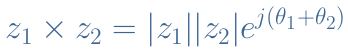
If z1 and z2 are written in exponential form, the multiplication operation is even easier to realize :
eq 7 : Multiplication using the exponential form
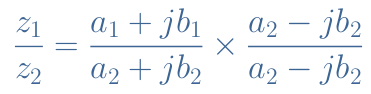
The division operation with complex numbers is however more complicated to perform, using the algebraic form than with real numbers. Let’s consider the two complex numbers z1 and z2 previously defined. The trick to perform a division is to transform the complex denominator into a real denominator. For this, we multiply both the numerator and denominator by the denominator complex conjugate such as shown below :
By realizing the multiplication such as shown previously, we get now a complex numerator that can be divided by a real denominator :
eq 8 : Division of two complex numbers
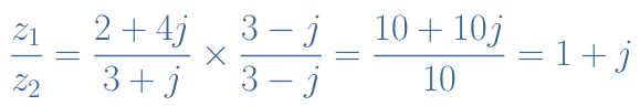
Let’s consider the example of z1=2+4j and z2=3+j and proceed to the division z1/z2 :
This result, can also be written in exponential form z1/z2=√2ejπ/4.
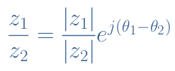
Such as we highlighted for the multiplication operation, the division can be done more easily with the exponential form :
eq 9 : Division using the exponential form
Equation 9 can be verified with the same example. First, we need to calculate the modules and arguments of z1 and z2 :
|z1|=√22+42=√20 and θ1=Arg(z1)=arctan(4/2)=arctan(2)
|z2|=√32+12=√10 and θ2=Arg(z2)=arctan(1/3)
The division of the modules gives |z1|/|z2|=√2 and the argument of the division is arctan(2)-arctan(1/3)=π/4. The result of the division is therefore √2ejπ/4 and confirms the result we previously calculated using the algebraic form.
Complex numbers in electronics
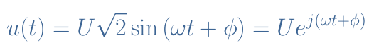
Any periodical signal such as the current or voltage can be written using the complex numbers that simplifies the notation and the associated calculations :
eq 10 : Complex notation for the voltage
The complex notation is also used to describe the impedances of capacitor and inductor along with their phase shift. It can indeed be shown that :
ZC=1/Cω and ΦC=-π/2
ZL=Lω and ΦL=+π/2
Since e±jπ/2=±j, the complex impedances Z* can take into consideration both the phase shift and the resistance of the capacitor and inductor :
ZC*=-j/Cω
ZL*=jLω
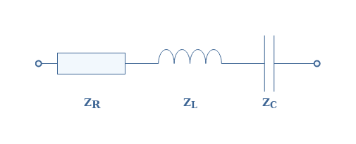
We can consider as an example a simple RLC circuit in serie with its associated complex impedances ZR, ZL and ZC. The total complex impedance is therefore : ZRLC=ZR+ZL+ZC=R+j(Lω-1/Cω).
The imaginary part of this impedance is called the reactance and noted X, in this example, XRLC=Lω-1/Cω. We can distinguish three cases to describe the behavior of a circuit :
X=0 means that the circuit is purely resistive : it acts as a resistance and follows Ohm’s law
X<0 the circuit is capacitive : it acts as a capacitance and tends to make an opposition to any change of voltage.
X>0 the circuit is inductive : it acts as a inductance and provokes an opposition to any change of current.
The total impedance of the RLC circuit is given by the module of ZRLC which is : |ZRLC|=√(R2+XRLC2).
The phase shift between the voltage and current is given by the argument of ZRLC which is : Arg(ZRLC)=arctan(XRLC/R).
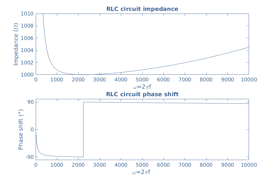
Both the impedance and phase shift depend on the frequency of the signals. This evolution can be represented using MatLab® in Figure 3 where the components have been chosen such as R=1 kΩ, L=10 mH, C=20 μF.
fig 3 : Impedance and phase shift of the RLC serie circuit. Plotted using MatLab®
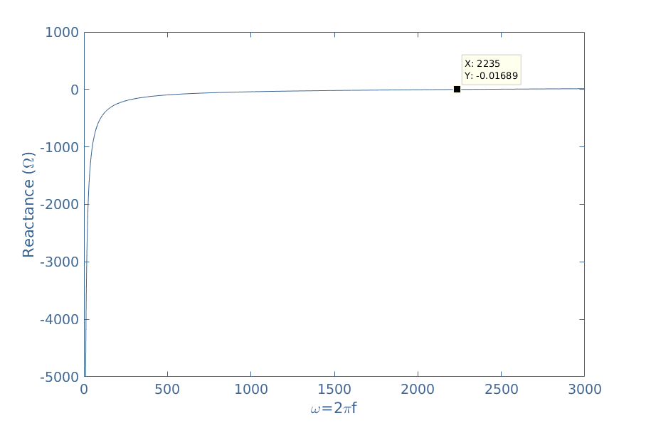
We can note that first the circuit is capacitive since it presents a negative phase shift and becomes inductive after a certain frequency value. This remark can be validated by plotting the reactance in Figure 4 where it is shown that the shift between negative and positive values occurs for the same particular frequency :
fig 4 : Reactance of the RLC serie circuit. Plotted using MatLab®
This particular frequency f0=2235/2π=356 Hz is called the resonance frequency of the circuit and satisfies X=0. In our example, XRLC=0 ⇒ ω0=1/√LC=2235, which is confirmed by the value highlighted in Figure 4.
Conclusion
Complex numbers have emerged since nearly 500 years and have been built by some of the most brilliant mathematicians such as Gauss or Cauchy. Since then, they are used in many scientific domains such as electronics and it’s a powerful tool.
In the very first section, the concept of complex numbers is presented. The complex set can be seen as a plane where each number can be defined by coordinates (algebraic form) or a distance and angle (exponential form). Complex numbers have the property to be solutions of some equations that cannot be solved by usual real numbers, such as the equation x2=-1. Some more important notions such as the conjugation transformation are introduced in a second section.
The calculation rules are presented in a third section. We have seen that the addition, subtraction and multiplication are very similar with real and complex numbers. However, the division operation requires more steps, involving the use of the conjugation transformation.
Finally, we have seen how complex numbers can be used in electronics to describe periodical signals, impedances and determine the behavior of circuits in frequency-dependent regimes.